Writing modular code with box

What is `box`?

box provides a precise and concise method for using add-on packages and functions. box also doesn’t require bundling your code into R packages to make it reusable. This post covers tackling some common workflow steps to demonstrate how box modules work.

Packages, functions, and namespaces

To understand the problem box solves, we’ll review the typical process for using add-on package functions in a standard R sesson and when developing R packages:

R sessions

Assume I want to use the glue() function from the glue package. The first step is to install it with install.packages("glue")
- I’ll use the example from the glue package website:
  show/hide
  
  install.packages("glue") # # The downloaded binary packages are in # /var/folders/0x/x5wkbhmx0k74tncn9swz7xpr0000gn/T//Rtmp2id54K/downloaded_packages
To use the functions from glue, I’ll need to run library(glue) in the same R session.
- If I try to use a function from a package but it hasn’t been attached with library or require, I see the following:
  show/hide
  
  name <- "Fred" glue('My name is {name}.') # Error in glue("My name is {name}."): could not find function "glue"
- The error above can be confusing, because it doesn’t tell us if the package hasn’t been installed, or if the package hasn’t been attached.
- However, after installing glue, I can get around using library by explicitly calling the function from the package namespace (i.e., pkg::foo()):
  show/hide
  
  name <- "Fred" glue::glue('My name is {name}.') # My name is Fred.
- While this method works, it doesn’t attach the package to the search list (which I check with search())
  show/hide
  
  base::search() # [1] ".GlobalEnv" "package:stats" "package:graphics" # [4] "package:grDevices" "package:utils" "package:datasets" # [7] "package:methods" "Autoloads" "package:base"
- library() attaches the glue package in the search list and makes the glue() function available to use (without the package:: prefix)
  show/hide
  
  library(glue) base::search() # [1] ".GlobalEnv" "package:glue" "package:stats" # [4] "package:graphics" "package:grDevices" "package:utils" # [7] "package:datasets" "package:methods" "Autoloads" # [10] "package:base"
- Unfortunately, library() also attaches all the objects from the glue package to the search() list, even though I’m only using a single function.

Read more about namespaces in Advanced R and R packages.

R packages

If I want to make the code I write using glue reusable, I can bundle it into an R package. Including glue as an add-on package (i.e., packages not loaded automatically with R) is done with the NAMESPACE file (created and edited via roxygen2 tags), and by listing these packages under Imports in the DESCRIPTION file.

In `R/` files:

All .R files in R packages are placed in the R/ folder. If these files use add-on packages (i.e., library() or package::fun()), I include the @import or @importFrom tag. If I’d like to include and make my_name() available to users, I use the @export tag:

I’ve converted the use of glue() into a small function below:

my_name() is saved as R/my_name.R:

show/hide

my_name <- function(x) {
  name <- x
  glue::glue('My name is {name}.')
}
my_name("Fred")
# My name is Fred.

Below is a default roxygen2 skeleton:

show/hide

#' Introduce yourself 
#'
#' @param x a name 
#'
#' @return An glued introduction to R
#' @export my_name
#'
#' @examples
#' my_name("Fred")
my_name <- function(x) {
  name <- x
  glue::glue('My name is {name}.')
}

As we can see, the default roxygen2 skeleton doesn’t include @import or @importFrom. The general advice is to prefer @importFrom over @import, because @import imports the entire package namespace (only use this in ‘very special situations’ such as ‘heavy use’ of a package functions).

Below is an example of using @importFrom:

show/hide

#' Introduce yourself 
#'
#' @param x a name 
#'
#' @return An glued introduction to R
#' @export my_name
#'
#' @examples
#' my_name("Fred")
#'
#' @importFrom glue glue
my_name <- function(x) {
  name <- x
  glue::glue('My name is {name}.')
}

NAMESPACE

While developing my R package, I’ll run devtools::load_all() and devtools::document() frequently, and each time the imported functions are available in the current session and the tags are converted into directives in the NAMESPACE file

import(package)
importFrom(package,function)

DESCRIPTION

A package DESCRIPTION file is managed completely independent of it’s NAMESPACE file. This can be confusing during package development, because it’s easy to assume some kind of connection between the roxygen2 tags, the NAMESPACE file, and the DESCRIPTION file:

However, this is not the case:
- To include glue in the DESCRIPTION under Imports, I also need to use usethis::use_package("glue")
- As noted in R packages, “The Imports field [in the DESCRIPTION file] makes sure that the packages listed there are installed when your package is installed.” The DESCRIPTION file does not make functions available to the package developer (or the user).

The recommended practices for add-on packages are 1) use the namespace-qualified calls in the R/ scripts (i.e., package::function() with an accompanying @importFrom package function tag), and 2) list these packages in the DESCRIPTION file under Imports or Suggests to make sure a package is installed whenever your package is installed (i.e., with usethis::use_package("package"))

The table below shows the connection between roxygen2 tags, the resulting NAMESPACE entry, and what should be listed in the DESCRIPTION (this is also covered in R packages)

Refresher on roxygen2, NAMESPACE & DESCRPTION

roxygen2 tag	NAMESPACE directive	DESCRIPTION
@importFrom	importFrom() : import selected object from another namespace	Consider listing under ‘Suggests’
@import	import(): import all objects from another package’s namespace	List under ‘Imports’
@export	export() : export the function, method, generic, or class so it’s available outside of the package (in the namespace)	Nothing to list

How `box` is different

box doesn’t require installing or attaching add-on packages. Instead, it uses modules to make package functions available. I’ll demonstrate with a simplified example using the glue() package. Assume I have a project folder pkg/,

show/hide

pkg/
  └── pkg.Rproj

1 directory, 1 file

Projects in RStudio have a hidden folder, .Rproj.user/:

The the following contents are automatically created with a new .Rproj file:

contents of .Rproj

pkg/
  ├── .Rproj.user
  │      ├── 8CC5F70E
  │      │      ├── bibliography-index
  │      │      ├── ctx
  │      │      ├── explorer-cache
  │      │      ├── presentation
  │      │      ├── profiles-cache
  │      │      ├── sources
  │      │      │      └── session-16ca0811
  │      │      │          └── lock_file
  │      │      ├── tutorial
  │      │      └── viewer-cache
  │      └── shared
  │          └── notebooks
  │              └── patch-chunk-names
  └── pkg.Rproj

14 directories, 3 files

None of these contents deal with installing or loading packages, but I’ve included it here for full transparency

Create a box module

I’ll put the modules in a box/fun.R file, which I’ll create from the command-line:

show/hide

mkdir box 
touch box/fun.R

Now my pkg folder looks like this:

show/hide

pkg/
  ├── box
  │    └── fun.R
  ├── pkg.Rproj
  └── use.R

2 directories, 3 files

In pkg/box/fun.R I’ll add the following:

a brief comment with the path to the module
the @export tag from roxygen2
a call to box::use(glue[glue])

show/hide

# box/fun.R
#' @export
box::use(
  glue[glue]
  )

In the parent folder, create another file named use.R.

In use.R, use the fun module by calling box::use(box/fun)

show/hide

box::use(box/fun)

View fun by printing it to the console:

show/hide

# print
fun

show/hide

<module: box/fun>

This confirms the module has been created.

Using modules

The glue function is available from fun using the $ (like a column in a data.frame or tibble)

show/hide

# use 
x <- "module"
fun$glue('This is a box {x}.')

show/hide

This is a box module.

box modules are combinations of named folders and files, but unlike R packages, these folders and files can be nested. The folder/file structure is used for separating modules, the same way we might separate files in a project (i.e., project/data/file.csv and project/code/analysis.R)

box makes the function and package namespacing explicit by using box::use(package[fun])
box also simplifies using module by calling the same function when building/using modules box::use(folder/file):

# CREATE MODULE
# box/fun.R
#' @export
box::use(
  glue[glue]
  )

# USE MODULE
box::use(box/fun)

Below is a slightly more involved example:

Module workflow

Below I’m going to create a module that imports, wrangles, and visualizes data from the palmerpenguins package. (which is installed, but not loaded).

`box/import`

This workflow starts with an import module in a pengbox project. The code below is stored in pengbox/box/import.R:

import module

# box/import.R
box::use(
  readr[read_csv],
)
#' @export
get_raw_csv <- function() {
  raw_csv_url <- "https://bit.ly/3SQJ6E3"
  read_csv(raw_csv_url)
}

In a the master pengbox/run.R file, I’ll use import like so:

show/hide

# import
box::use(box/import)
str(import$get_raw_csv(), give.attr = FALSE)

show/hide

spc_tbl_ [344 × 17] (S3: spec_tbl_df/tbl_df/tbl/data.frame)
 $ studyName          : chr [1:344] "PAL0708" "PAL0708" "PAL0708" "PAL0708" ...
 $ Sample Number      : num [1:344] 1 2 3 4 5 6 7 8 9 10 ...
 $ Species            : chr [1:344] "Adelie Penguin (Pygoscelis adeliae)" "Adelie" ...
 $ Region             : chr [1:344] "Anvers" "Anvers" "Anvers" "Anvers" ...
 $ Island             : chr [1:344] "Torgersen" "Torgersen" "Torgersen" 
 $ Stage              : chr [1:344] "Adult, 1 Egg Stage" "Adult, 1 Egg Stage" 
 $ Individual ID      : chr [1:344] "N1A1" "N1A2" "N2A1" "N2A2" ...
 $ Clutch Completion  : chr [1:344] "Yes" "Yes" "Yes" "Yes" ...
 $ Date Egg           : Date[1:344], format: "2007-11-11" "2007-11-11" ...
 $ Culmen Length (mm) : num [1:344] 39.1 39.5 40.3 NA 36.7 39.3 38.9 ...
 $ Culmen Depth (mm)  : num [1:344] 18.7 17.4 18 NA 19.3 20.6 17.8 19.6 ...
 $ Flipper Length (mm): num [1:344] 181 186 195 NA 193 190 181 195 193 ...
 $ Body Mass (g)      : num [1:344] 3750 3800 3250 NA 3450 ...
 $ Sex                : chr [1:344] "MALE" "FEMALE" "FEMALE" NA ...
 $ Delta 15 N (o/oo)  : num [1:344] NA 8.95 8.37 NA 8.77 ...
 $ Delta 13 C (o/oo)  : num [1:344] NA -24.7 -25.3 NA -25.3 ...
 $ Comments           : chr [1:344] "Not enough blood for isotopes." NA NA ...

I’ll re-write this module in box/import.R using an alias for readrs read_csv() function (rcsv) and include the readr::cols() function to remove the lengthy message.

This code is stored in the box/import.R file:

import module with alias

# box/import.R
box::use(
  readr[rcsv = read_csv, cols]
)
#' @export
raw <- function() {
  raw_csv_url <- "https://bit.ly/3SQJ6E3"
  # use alias for read_csv()
  rcsv(raw_csv_url, col_types = cols())
}

Using import with the new module is more concise:

show/hide

# import
box::use(box/import)
str(import$raw(), give.attr = FALSE)

show/hide

spc_tbl_ [344 × 17] (S3: spec_tbl_df/tbl_df/tbl/data.frame)
 $ studyName          : chr [1:344] "PAL0708" "PAL0708" "PAL0708" "PAL0708" ...
 $ Sample Number      : num [1:344] 1 2 3 4 5 6 7 8 9 10 ...
 $ Species            : chr [1:344] "Adelie Penguin (Pygoscelis adeliae)" "Adelie" ...
 $ Region             : chr [1:344] "Anvers" "Anvers" "Anvers" "Anvers" ...
 $ Island             : chr [1:344] "Torgersen" "Torgersen" "Torgersen" 
 $ Stage              : chr [1:344] "Adult, 1 Egg Stage" "Adult, 1 Egg Stage" 
 $ Individual ID      : chr [1:344] "N1A1" "N1A2" "N2A1" "N2A2" ...
 $ Clutch Completion  : chr [1:344] "Yes" "Yes" "Yes" "Yes" ...
 $ Date Egg           : Date[1:344], format: "2007-11-11" "2007-11-11" ...
 $ Culmen Length (mm) : num [1:344] 39.1 39.5 40.3 NA 36.7 39.3 38.9 ...
 $ Culmen Depth (mm)  : num [1:344] 18.7 17.4 18 NA 19.3 20.6 17.8 19.6 ...
 $ Flipper Length (mm): num [1:344] 181 186 195 NA 193 190 181 195 193 ...
 $ Body Mass (g)      : num [1:344] 3750 3800 3250 NA 3450 ...
 $ Sex                : chr [1:344] "MALE" "FEMALE" "FEMALE" NA ...
 $ Delta 15 N (o/oo)  : num [1:344] NA 8.95 8.37 NA 8.77 ...
 $ Delta 13 C (o/oo)  : num [1:344] NA -24.7 -25.3 NA -25.3 ...
 $ Comments           : chr [1:344] "Not enough blood for isotopes." NA NA ...

`box/prep`

After importing the raw penguins data, I’ll write a module for wrangling the data (that also imports the import module).

This module takes the following steps:

Reset the box.path
Import the box/import module
Load all the functions from dplyr using [...]
Load aliases for stringr::str_extract() and janitor::clean_names()
Compose prep() with the wrangling steps

prep module with import

# box/prep.R

# reset the path
options(box.path = getwd())

# import alias import module
box::use(box/import)

# wrangle packages, functions, and aliases
box::use(
  dplyr[...],
  stringr[str_ext = str_extract],
  janitor[fix_cols = clean_names]
)

#' @export
prep = function() {
  raw <- import$raw()
  clean_cols <- fix_cols(raw)
  vars <- select(clean_cols, 
    species, 
    island, 
    bill_length_mm = culmen_length_mm,
    bill_depth_mm = culmen_depth_mm,
    flipper_length_mm,
    body_mass_g,
    sex)
  mutate(vars, 
    species = str_ext(species, "([[:alpha:]]+)"),
    sex = factor(sex))
}

We can now the prep module to access the import module for the wrangled dataset.

# prepare
box::use(box/prep)
peng_clean <- prep$prep()
str(peng_clean, give.attr = FALSE)

tibble [344 × 7] (S3: tbl_df/tbl/data.frame)
 $ species          : chr [1:344] "Adelie" "Adelie" "Adelie" "Adelie" ...
 $ island           : chr [1:344] "Torgersen" "Torgersen" "Torgersen" "Torgersen" ...
 $ bill_length_mm   : num [1:344] 39.1 39.5 40.3 NA 36.7 39.3 38.9 39.2 34.1 42 ...
 $ bill_depth_mm    : num [1:344] 18.7 17.4 18 NA 19.3 20.6 17.8 19.6 18.1 20.2 ...
 $ flipper_length_mm: num [1:344] 181 186 195 NA 193 190 181 195 193 190 ...
 $ body_mass_g      : num [1:344] 3750 3800 3250 NA 3450 ...
 $ sex              : Factor w/ 2 levels "FEMALE","MALE": 2 1 1 NA 1 2 1 2 NA NA ...

These data look like they’re ready for graphing! Time to write another module…

`box/plot`

I will build my visualization with ggplot2 (in the box/plot.R module) and dplyr::filter():

plot module with prep

# pengbox/plot.R

# reset the path
options(box.path = getwd())

# import prep module
box::use(box/prep)

# import ggplot2
box::use(
  dplyr[filter],
  ggplot2 = ggplot2[ggplot, aes, geom_point, 
                    facet_wrap, labs, theme_minimal])

#' @export
scatter <- function() {
  prepped <- prep$prep()
  # remove missing sex
  filtered <- filter(prepped, !is.na(sex)) 
    # plot filtered data
  plotted <- ggplot2$ggplot(data = filtered, 
    ggplot2$aes(
      x = flipper_length_mm,
      y = body_mass_g,
      group = sex
    )
  ) +
    ggplot2$geom_point(
      ggplot2$aes(color = island)
    ) +
    ggplot2$facet_wrap(. ~ sex) +
    ggplot2$labs(x = "Flipper Length (mm)", y = "Body Mass (g)", 
      color = "Island", title = "Flipper vs. Body Mass", 
      subtitle = "Palmer Penguins") +
    ggplot2$theme_minimal()
  plotted
}

Check our scatter plot with plot$scatter()

show/hide

# plot
box::use(box/plot)
plot$scatter()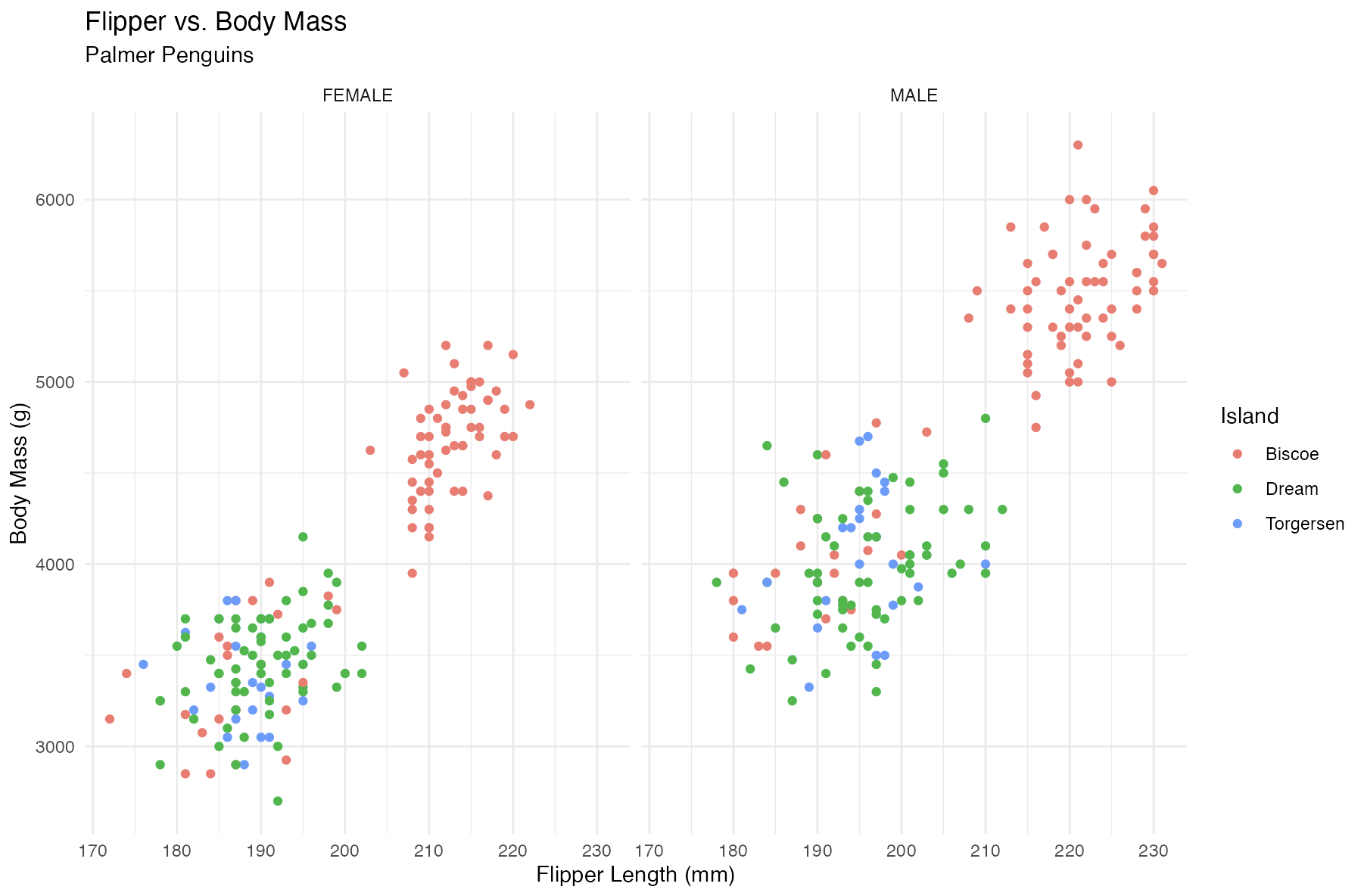

And there you have it! A complete pipeline using box modules! And the total project size (files and folders) is much smaller than building an R package:

show/hide

pengbox/
    ├── box
    │   ├── import.R
    │   ├── plot.R
    │   └── prep.R
    ├── penguins.Rproj
    └── run.R

2 directories, 5 files

Below are the various ways to include packages and functions in box modules:

Options for creating box modules:

Inside box::use()	Action
box::use( pkg )	\|imports ‘pkg’, does not attach any function names
box::use( p = pkg )	\|imports ‘pkg’ with alias (‘p’), does not attach any function names
box::use( pkg = pkg[foo, bar] )	\|imports ‘pkg’ and attaches the function names ‘pkg::foo()’ and ‘pkg::bar()’
box::use( pkg[my_foo = foo, …]	\|imports ‘pkg’ with alias for ‘foo’ (‘my_foo’) and attaches all exported function name

Nesting modules

The same workflow could be re-written as nested modules, with folders separating logical steps in an analysis workflow (or application). Consider the folder structure below:

show/hide

pengbox/
    ├── box
    │   └── graph
    │       ├── wrangle
    │       │   ├── clean
    │       │   │   ├── import
    │       │   │   │   └── raw.R
    │       │   │   └── cols.R
    │       │   └── vars.R
    │       └── scatter.R
    ├── penguins.Rproj
    └── run.R

6 directories, 6 files

`import`

With this structure, the raw module is in the import folder:

show/hide

pengbox/box/graph/wrangle/clean/import
                                    └── raw.R

1 directory, 1 file

The raw module–the first step–is nested in the box/graph/wrangle/clean/import/raw.R file

The raw module imports the raw .csv data with an aliass for readr’s read_csv()

raw module

# box/graph/wrangle/clean/import/raw.R
box::use(
  readr[rcsv = read_csv, cols]
)
#' @export
csv <- function() {
  raw_csv_url <- "https://bit.ly/3SQJ6E3"
  # use alias for read_csv()
  rcsv(raw_csv_url, col_types = cols())
}

`raw`

In run.R, I run box/graph/wrangle/clean/import/raw to import the raw module

The csv() function imports the raw data

show/hide

# in use.R
box::use(box/graph/wrangle/clean/import/raw)
str(raw$csv(), give.attr = FALSE)

raw module output

spc_tbl_ [344 × 17] (S3: spec_tbl_df/tbl_df/tbl/data.frame)
 $ studyName          : chr [1:344] "PAL0708" "PAL0708" "PAL0708" "PAL0708" ...
 $ Sample Number      : num [1:344] 1 2 3 4 5 6 7 8 9 10 ...
 $ Species            : chr [1:344] "Adelie Penguin (Pygoscelis adeliae)" "Adelie" ...
 $ Region             : chr [1:344] "Anvers" "Anvers" "Anvers" "Anvers" ...
 $ Island             : chr [1:344] "Torgersen" "Torgersen" "Torgersen" 
 $ Stage              : chr [1:344] "Adult, 1 Egg Stage" "Adult, 1 Egg Stage" 
 $ Individual ID      : chr [1:344] "N1A1" "N1A2" "N2A1" "N2A2" ...
 $ Clutch Completion  : chr [1:344] "Yes" "Yes" "Yes" "Yes" ...
 $ Date Egg           : Date[1:344], format: "2007-11-11" "2007-11-11" ...
 $ Culmen Length (mm) : num [1:344] 39.1 39.5 40.3 NA 36.7 39.3 38.9 ...
 $ Culmen Depth (mm)  : num [1:344] 18.7 17.4 18 NA 19.3 20.6 17.8 19.6 ...
 $ Flipper Length (mm): num [1:344] 181 186 195 NA 193 190 181 195 193 ...
 $ Body Mass (g)      : num [1:344] 3750 3800 3250 NA 3450 ...
 $ Sex                : chr [1:344] "MALE" "FEMALE" "FEMALE" NA ...
 $ Delta 15 N (o/oo)  : num [1:344] NA 8.95 8.37 NA 8.77 ...
 $ Delta 13 C (o/oo)  : num [1:344] NA -24.7 -25.3 NA -25.3 ...
 $ Comments           : chr [1:344] "Not enough blood for isotopes." NA NA ...

`clean`

The clean folder contains the cols module and the snakes() function

show/hide

box/graph/wrangle/
              ├── clean
              │   ├── #import
              │   │   #└── raw.R
              │   └── cols.R
              └── vars.R

3 directories, 3 files

`snakes`

The box/graph/wrangle/clean/cols module standardizes the column names

cols calls the snakes() function, which converts all the column names to lower_snake_case with an alias for janitor::clean_names(), then it imports select from dplyr to subset the columns

cols module

# box/graph/wrangle/clean/cols.R

# reset the path
options(box.path = getwd())

# use import raw module
box::use(box/graph/wrangle/clean/import/raw)

# columns
box::use(
  dplyr[select],
  janitor[fix_cols = clean_names]
)

#' @export
snakes = function() {
  raw <- raw$csv()
  clean_cols <- fix_cols(raw)
  vars <- select(clean_cols, 
    species, 
    island, 
    bill_length_mm = culmen_length_mm,
    bill_depth_mm = culmen_depth_mm,
    flipper_length_mm,
    body_mass_g,
    sex)
  return(vars)
}

Back in run.R, we call the cols module to convert the columns names with snakes():

# clean columns
box::use(box/graph/wrangle/clean/cols)
names(cols$snakes())

cols module output

[1] "species"           "island"            "bill_length_mm"    "bill_depth_mm"                  
[5] "flipper_length_mm" "body_mass_g"       "sex"

`wrangle`

Now that I have standardized columns and the subset of the variables to plot, I can call the vars module to wrangle the plot variables

show/hide

box/graph/wrangle/
            ├── #clean
            │   #├── #import
            │   #│   #└── raw.R
            │   #└── cols.R
            └── vars.R

3 directories, 3 files

`vars`

vars is nested in the wrangle folder, and imports the raw and cols modules

The vars module imports mutate and filter from dplyr and an alias for stringr::str_extract()

vars module

# box/graph/wrangle/vars.R

# reset the path
options(box.path = getwd())

# use clean names module
box::use(box/graph/wrangle/clean/cols)

# wrangle packages/functions
box::use(dplyr[mutate, filter],
  stringr[str_ext = str_extract])

#' @export
scatter = function() {
  clean_cols <- cols$snakes()
  plot_vars <- clean_cols |>
    mutate(
      species = str_ext(species, "([[:alpha:]]+)"),
      species = factor(species),
      island = factor(island),
      sex = factor(sex)
    ) |>
    # remove missing sex
    filter(!is.na(sex))
  return(plot_vars)
}

In run.R, we check the structure of the output from vars$scatter()

show/hide

# in run.R
# wrangle variables 
box::use(box/graph/wrangle/vars)
str(vars$scatter())

vars module output

tibble [333 × 7] (S3: tbl_df/tbl/data.frame)                                                     
 $ species          : Factor w/ 3 levels "Adelie","Chinstrap",..: 1 1 1 1 1 1 1 1 1 1 ...
 $ island           : Factor w/ 3 levels "Biscoe","Dream",..: 3 3 3 3 3 3 3 3 3 3 ...
 $ bill_length_mm   : num [1:333] 39.1 39.5 40.3 36.7 39.3 38.9 39.2 41.1 38.6 34.6 ...
 $ bill_depth_mm    : num [1:333] 18.7 17.4 18 19.3 20.6 17.8 19.6 17.6 21.2 21.1 ...
 $ flipper_length_mm: num [1:333] 181 186 195 193 190 181 195 182 191 198 ...
 $ body_mass_g      : num [1:333] 3750 3800 3250 3450 3650 ...
 $ sex              : Factor w/ 2 levels "FEMALE","MALE": 2 1 1 1 2 1 2 1 2 2 ...

`graph`

Finally, we get to the graph module. This module import all preceding modules.

box/
└── graph
    ├── #wrangle
    │   #├── #clean
    │   #│   #├── #import
    │   #│   #│   #└── raw.R
    │   #│   #└── cols.R
    │   #└── vars.R
    └── scatter.R

5 directories, 4 files

`scatter`

The scatter module imports the vars module with the data that’s been imported, cleaned, and wrangled.

The ggp2() function includes the ggplot2 functions to build a scatter plot.

scatter module

# box/graph/scatter.R

# reset the path
options(box.path = getwd())

# import plot vars module
box::use(box/graph/wrangle/vars)

# import ggplot2
box::use(
  ggplot2 = ggplot2[ggplot, aes, geom_point, 
                    facet_wrap, labs, theme_minimal]
)

#' @export
ggp2 <- function() {
  scatter_vars <- vars$scatter()
  # plot prepped data
  ggp2_plot <- ggplot2$ggplot(data = scatter_vars, 
    ggplot2$aes(
      x = flipper_length_mm,
      y = bill_length_mm,
      group = island
    )
  ) +
    ggplot2$geom_point(
      ggplot2$aes(color = species)
    ) +
    ggplot2$facet_wrap(. ~ island) +
    ggplot2$labs(
      x = "Flipper Length (mm)", 
      y = "Bill length (mm)", 
      color = "Species",
      group = "Island",
      title = "Flipper vs. Bill Length", 
      subtitle = "Palmer Penguins"
    ) +
    ggplot2$theme_minimal()
  ggp2_plot
}

In run.R, the final module call produces the plot.

# graph
box::use(box/graph/scatter)
scatter$ggp2()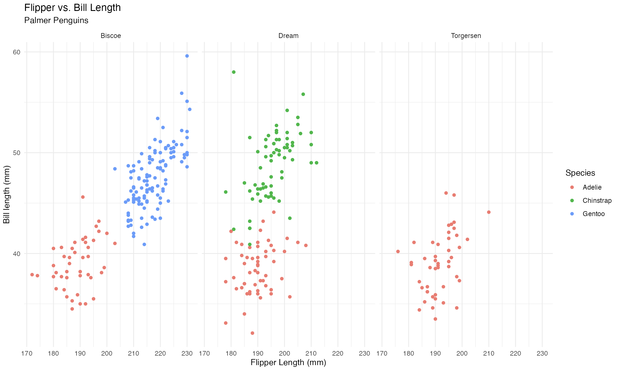

Recap

In this post I’ve covered how the box package uses modules to separate your analysis and workflow into small, modular scripts. Nesting modules also adds a flexibility R packages do not have (because everything has to be contained in the R/ folder).

Both versions of the projects created in this example ended up with very few lines of code, and didn’t require a creating a NAMESPACE or DESCRIPTION file.

View the final project here.

What is box?

Packages, functions, and namespaces

R sessions

R packages

In R/ files:

NAMESPACE

DESCRIPTION

How box is different

Create a box module

Using modules

Module workflow

box/import

box/prep

box/plot

Nesting modules

import

raw

clean

snakes

wrangle

vars

graph

scatter

Recap

What is `box`?

In `R/` files:

How `box` is different

`box/import`

`box/prep`

`box/plot`

`import`

`raw`

`clean`

`snakes`

`wrangle`

`vars`

`graph`

`scatter`