packages
library(testthat)
library(lobstr)
library(dplyr)
library(shiny)
library(covr)library(testthat)
library(lobstr)
library(dplyr)
library(shiny)
library(covr)This post is the first in a series on testing Shiny applications. We’ll cover developing and testing a set of utility functions for a Shiny app-package using testhat. If you’d like to follow along, all the code we’ll be using is contained in the utap branch of the sapkgs repo on GitHub.
# renv::install("mjfrigaard/utap")
library(utap)
Testing the code in Shiny app-packages can be more complicated than testing the code in a typical R package, because app-packages contain two types of code:
Application code: functions designed to run the application (i.e., the ui and server functions, modules, standalone app functions will a call to shinyApp(), etc.)
Everything else: functions or code used for connecting to databases, uploading, importing, or manipulating data, building visualizations and/or tables, generating custom HTML layouts, etc. The non-application code and functions in app-packages are typically referred to as ‘utility’ or ‘helper’ functions
These two types of code require different types of tests. Utility functions are usually accompanied by unit tests similar to the tests you’d find in a standard R package1, while the application’s reactive code can be tested using Shiny’s testServer() function, and the system tests can be built using the shinytest2 package.
This post will cover writing unit tests for a set of utility functions using testthat and covr. Any tips or time-savers I’ve found will be in green callout boxes:

“A unit test is a piece of code that invokes a unit of work and checks one specific end result of that unit of work. If the assumptions on the end result turn out to be wrong, the unit test has failed. A unit test’s scope can span as little as a method or as much as multiple classes.” - The Art of Unit Testing, 2nd edition
Thinking of functions as ‘units of work’ and their desired behavior as an ‘end results’ provides a useful mental model (especially during behavior-driven development. These terms also align nicely with the testing advice offered by testthat:
Strive to test each behaviour in one and only one test. Then if that behaviour later changes you only need to update a single test.
In app-packages, the testthat package provides a comprehensive and flexible framework for performing unit tests.
Get started with testthat by running usethis::use_testthat(). This function will create following files and folders:
tests/
  ├── testthat/
  └── testthat.R
To create new tests, we’ll run usethis::use_test("<name>") (with "select_class" being the name of the function we’d like to test).
usethis::use_test("select_class")✔ Setting active project to '/projects/apps/utap'
✔ Writing 'tests/testthat/test-select_class.R'
• Modify 'tests/testthat/test-select_class.R'New test files are be created and opened from the tests/testthat/ folder (with a test- prefix). Each function we’re testing should have it’s own .R file the R/ folder and a corresponding test- file in the tests/testthat/ folder (we’ll see how this helps with interactive testing in the IDE below). The initial contents of a new test file contains the boilerplate code below:
test_that("multiplication works", {
  expect_equal(2 * 2, 4)
})
test_that() sets the test “scope” or “execution environment”, and encapsulates the test code and expectations. Note the use of curly brackets after the code argument:
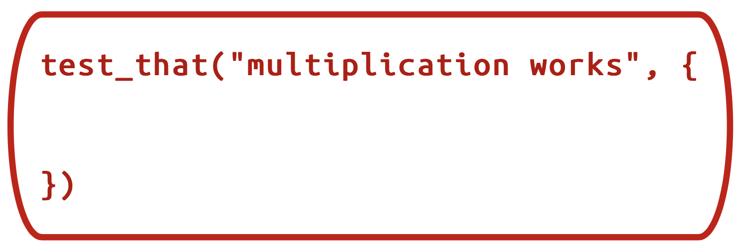
testthat test
Test expectations are the code that comes into direct contact with the unit of work and end result for each function. It’s likely we’ll have multiple expectations for any given function, so we store these in tests and use the desc to describe the test context (all testthat expectations have an expect_* prefix):
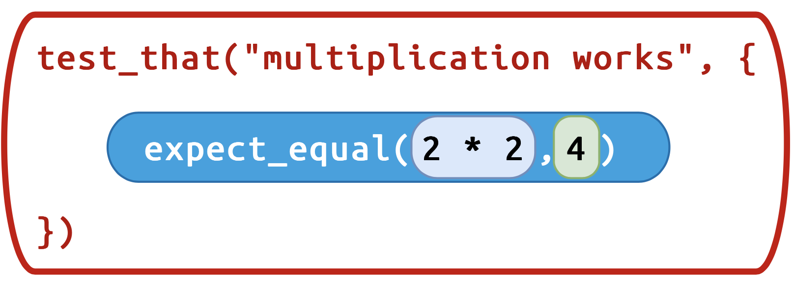
expect_* functions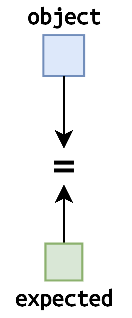
I highly recommend using a shortcut while developing tests because it will improve your ability to iterate quickly.2
devtools functiontest()
Ctrl/Cmd + Shift + T
test_active_file()
Ctrl/Cmd + T
test_coverage_active_file()
Ctrl/Cmd + Shift + R
Behavior-driven development (or behavior-driven testing) is helpful if you find yourself communicating with users and/or stakeholders while developing Shiny apps. BDD centers around “conversation and examples to specify how you expect a system to behave”3 and it’s supported with testthats describe() and it() functions.4
In R packages, micro-iteration is defined as, “the interactive phase where you initiate and refine a function and its tests in tandem.” In app development, this stage might after you’ve received needs or specifications by an end-user or stakeholder.
If we’re using BDD, we’ll translate these specifications into functional requirements, then start writing test(s). After outlining the tests, we’ll write the function(s) to pass the test.
testthat’s describe() and it() functions and Gherkin syntax can clarify this process because we can describe what it is we want to test before getting stuck writing any test code.
Let’s assume we’ve been asked to design an application that automatically to populates the user drop-downs with variables based on their format: binary, numeric, categorical, and–a subset of categorical–facet.5
description (entered as a character string in the first argument of describe()) to capture the “unit of work” for each function. Feature and Background information can be included in nested describe() blocks.describe("
Feature: Pull column names by type from a data frame or tibble
Background: Given a data frame or tibble
And it has binary, character, and numeric columns", code = {
})Scenario keyword should have a corresponding it() or test_that() call.6 Try to be as specific as possible (while staying short and sweet) when describing the scenarios.describe("
Feature: Pull column names by type from a data frame or tibble
Background: Given a data frame or tibble
And it has binary, character, and numeric columns", code = {
it("Scenario: Given a data frame with a mix of columns
When I call pull_cols() with type 'binary'
Then I should receive a list of 'binary' column names", code = {
})
})Then keywords capture our expectations (and expect_*() function). In this case, it’s the ‘list of column names that match the "<type>" criteria’describe("
Feature: Pull column names by type from a data frame or tibble
Background: Given a data frame or tibble
And it has binary, character, and numeric columns", code = {
it("Scenario: Given a data frame with a mix of columns
When I call pull_cols() with type 'binary'
Then I should receive a list of 'binary' column names", code = {
expect_equal(is.logical(object))
})
})It’s worth noting that, at least conceptually, scenarios and expectations arise first. We’re usually working backwards from a desired “end result” a function is supposed to produce (i.e., compute a value, download a file, create a column, etc.).
For example, calling pull_cols(df, "bin") would ‘pull’ all the binary columns from an input data.frame or tibble (the example below uses palmerpenguins::penguins):
pull_cols(palmerpenguins::penguins, type = "bin")## sex
## "sex" The return values can be passed to updateSelectInput() in the server to provide column names by type (i.e., numeric, binary, etc). pull_colls() can be used to quickly group variables into groups for data visualizations or table displays.
For example, categorical variables with 3-5 levels can be mapped to a facet layer (if using ggplot2). See the hypothetical UI output example below:
# UI code
selectInput(
inputId = ns("facet"),
label = "Select Facet Column",
choices = c("", NULL)
)# pull facet columns from data
facet_cols <- reactive({
pull_cols(df = ds(), type = "facet")
})
# update facet inputs
observe({
updateSelectInput(
session = session,
inputId = "facet",
choices = facet_cols()
)
}) |>
bindEvent(facet_cols())In the example above, pull_cols() is passed a reactive dataset (data()), and the output is used to update the selectInput():
The first step of pull_cols() will be to identify and extract columns based on their class, so we’ll create a test for select_class(), a function with a class parameter that supports multiple column types. The roxygen2 documentation for select_class() is below:
#' Select Column Class
#'
#' `select_class()` selects columns from a data.frame based on the specified
#' `class`. Options include logical, integer, double, character, factor, ordered,
#' and list column types.
#'
#' @param df A `data.frame` from which columns will be selected.
#' @param class Character vector specifying the class(es) of columns to select.
#' Supported values are:
#' * "logical" ("lo")
#' * "integer" ("in")
#' * "double" ("do")
#' * "character" ("ch")
#' * "factor" ("fa")
#' * "ordered" ("or")
#' * "list" ("li")
#'
#' @param return_tbl Logical indicating whether to return the result as a
#' `data.frame`. If `FALSE`, a vector of selected column names is returned.
#'
#' @return A `data.frame` or vector of column names, depending on `return_tbl`.We’ve also included a return_tbl argument that allows select_class() to return the column names.
While developing R functions, I’ve found the ast() function from the lobstr package can be great for keeping track of nested function calls.
select_class() will have a nested is_class() function, which contains a series of test for objects (i.e., is.logical(), is.integer(), etc.). To keep track of nested functions in R/ files, sometimes I’ll outline the function in an abstract function tree and store this in a vignette.7
Below is an example tree for select_class():
Syntax:
lobstr::ast(
select_class(
is_class()
)
)Output:
█─select_class
└─█─is_class The tree above is simple–it only has two functions so far–but as packages grow these abstract displays become more important for tracking function calls (and tests!).
Outlining functions with lobstr::ast() can helpful if we plan on iterating multiple, smaller functions. For example, before making a binary vector of column names, we need to verify the column has only two values. Binary variables can come in multiple flavors (logical, integer, character, factor, ordered, etc.), so check_binary_vec() will have a series of ‘checks’ for each column type.
Below is an abstract folder tree outlining pull_binary_cols(), the function called to extract a named character vector of binary column names:
█─pull_binary_cols
├─█─select_class
│ └─█─is_class
└─█─make_binary_vec
└─█─check_binary_vec
├─█─check_log_binary
├─█─check_int_binary
├─█─check_chr_binary
├─█─check_fct_binary
└─█─check_ord_binary pull_binary_cols() calls select_class() then passes the selected columns to make_binary_vec(), where check_binary_vec() determines if it’s one of the five types of possible binary variables.
pull_binary_cols(palmerpenguins::penguins)
##  sex
## "sex"pull_binary_cols(dplyr::starwars)
## gender
## "gender"The pull_facet_cols() outline is similar, except that it calls the pull_binary_cols() first, then selects the columns and determines if any remaining have 3-5 categorical levels:
█─pull_facet_cols
├─█─pull_binary_cols
├─█─select_class
│ └─█─is_class
└─█─make_facet_vec
  └─█─check_facet_vec
    ├─█─check_chr_facet
└─█─check_fct_facet Before we can start developing the tests for pull_cols(), we’ll need data. We can define test data inside the it() call for select_class():
describe("select_class() returned objects", code = {
it("df returned", {
# define test data
test_data <- data.frame(
log_var = c(TRUE, FALSE, TRUE),
int_var = c(1L, 2L, 3L),
dbl_var = c(1.1, 2.2, 3.3),
chr_var = paste0(rep("item:", times = 3), 1:3))
})
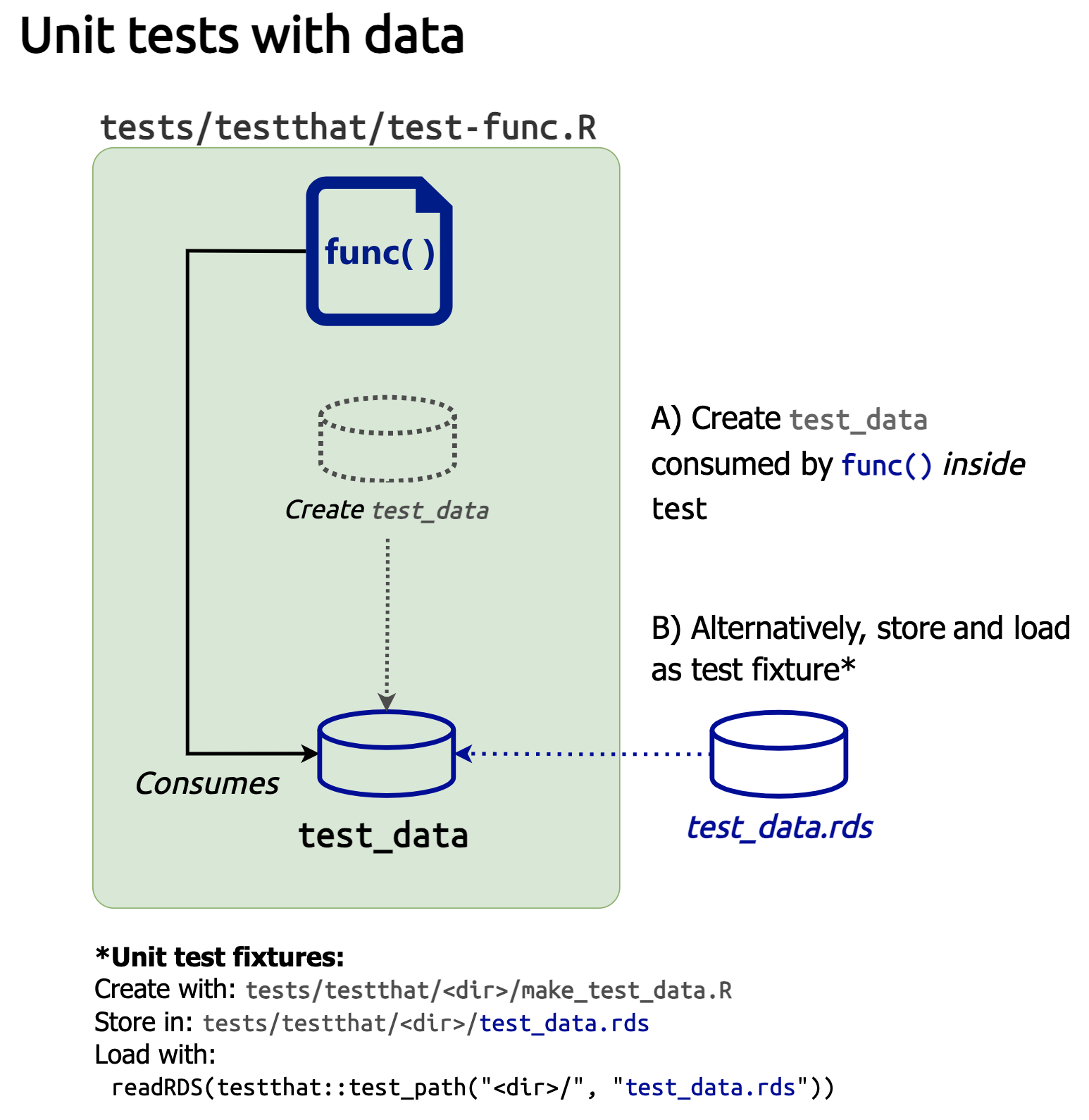
})This is helpful because it’s clear what test_data contains, and many times a small dataset will suffice. However, larger, more complex test data should be stored as a test fixture.
Creating test fixtures is covered in R packages, but I’ll summarize the key points:
Test data (and other objects) can either be created within a test, or as a persistent test fixture
Test data fixtures should be stored in tests/testthat/fixtures/<test_data.rds>
The code used to create any test data fixtures should be stored in the same folder with a make_ prefix (i.e., tests/testthat/fixtures/<make_test_data.R>)
This is easier to picture with a demonstration: In the tests/testthat/ folder, I’ll create a new fixtures folder, and add a make_test_data.R file.8
tests/testthat/
        └── fixtures/
                └── make_test_data.R
In make_test_data.R, I’ll create test_data using the code above and save test_data in tests/testthat/fixtures/ as test_data.rds:
tests/testthat/
        └── fixtures/
                ├── make_test_data.R
                └── test_data.rds
To load the data into my test, I’ll add the following to the top of the test context:
describe("select_class() returned objects", code = {

  test_data <- readRDS(test_path("fixtures", "test_data.rds"))

})
testthat::test_path() will load the data from the testing directory when I’m ready to run my test.
The select_class() function should also be able to return a data.frame/tibble of the specified class, or a named vector of the column names. testthat’s expect_* functions have a lot of options for writing very specific tests.
describe("select_class() returned objects", code = {

  it("df returned", {
    # define/load test data
    expect_s3_class(object, "data.frame")
  })

  it("tibble returned", {
    # define/load test data
    expect_s3_class(object,
      class = c("tbl_df", "tbl", "data.frame")
    )
  })

  it("string returned", {
    # define/load test data
    expect_type(object = object, type = "character")
  })

  it("named vector returned", {
    # define/load test data
    expect_named(object = object, expected = "log_var")
  })
})
select_class() should also return the columns according to the class argument. For the logical, integer, double, character, and list columns, we can assess each returned object with expect_type(). However, with the factor and ordered columns, we’ll use the expect_s3_class().
# check classes ----
describe("select_class() return classes", code = {
  ## check logical ----
    it("logical works", {
      test_data <- readRDS(test_path("fixtures", "test_data.rds"))
      # define obj
      obj <- select_class(df = test_data, class = "logical")
      # test type
      expect_type(obj[[1]], type = "logical")
    })
    ## check integer ----
    it("integer works", {
      # integer test code
      })
  ## check double ----
    it("double works", {
      # double test code
    })
  ## check character ----
    it("character works", {
      # character test code
    })
    ## check list ----
    it("list works", {
      # list test code
    })
  ## check factor ----
    it("factor works", {
      test_data <- readRDS(test_path("fixtures", "test_data.rds"))
      obj <- select_class(df = test_data, class = "factor")
      expect_s3_class(obj[[1]], class = "factor")
    })
  ## check factor (ordered) ----
    it("ordered works", {
      # ordered factor test code
    })

})
Using describe() and it() allows us to outline tests for select_class(), and including test fixtures makes it easier to test all possible classes returned.
When we’ve covered my intended ‘end results’ for select_class() (i.e., what we expect to happen when it works and we expect to happen when it doesn’t), we cam write the function:
select_class <- function(df, class, return_tbl = TRUE) {
  if (!is.data.frame(df)) stop("df must be a dataframe")

  # define classes
  valid_classes <- c("logical", "integer", "double", "numeric", "character",
                     "factor", "ordered", "list")
  class <- match.arg(class, choices = valid_classes, several.ok = TRUE)

  # helper function to check classes
  is_class <- function(x, cls) {
    cls <- match(cls, valid_classes)
    cls_name <- valid_classes[cls]
    switch(cls_name,
           logical = is.logical(x),
           integer = is.integer(x),
           double = is.double(x),
           numeric = is.numeric(x),
           character = is.character(x),
           factor = is.factor(x),
           ordered = is.ordered(x),
           list = is.list(x),
           FALSE)
  }

  selected_cols <- sapply(df, function(x) any(sapply(class, is_class, x = x)))

  col_names <- names(df)[selected_cols]

  if (return_tbl) {
    return(df[, col_names, drop = FALSE])
  } else {
    return(setNames(object = col_names, nm = col_names))
  }
}
Below is a summary of tips for adding data your tests.
Test helpers can be stored in tests/testthat/helper.R. Test helpers are functions or code that 1) is too long to repeat with each test, and 2) doesn’t take too much time or memory to run. Read more about test helpers here..
For this application, I’ve created a set of test helpers to make different forms of test data (because we’ll be repeatedly defining columns with slightly different attributes).
For example, col_maker() can be used to create a tibble with columns based on the col_type, size, and missing:
col_maker(col_type = c("log", "int", "dbl",
                       "chr", "fct", "ord"),
          size = 3,
          missing = TRUE)
## # A tibble: 3 × 6
##   log_var int_var dbl_var chr_var fct_var ord_var
##   <lgl>     <int>   <dbl> <chr>   <fct>   <ord>
## 1 TRUE          1     0.1 item:1  group 1 level 1
## 2 FALSE        20    NA   <NA>    <NA>    <NA>
## 3 NA           NA     0.1 item:1  group 1 level 1
I can also create tibbles with custom columns using individual helper _maker() functions:
tibble::tibble(
    log_var = log_maker(size = 3),
    chr_var = chr_maker(size = 3, lvls = 3),
    ord_var = ord_maker(size = 3, lvls = 2)
)
## # A tibble: 3 × 3
##   log_var chr_var ord_var
##   <lgl>   <chr>   <ord>
## 1 TRUE    item:1  level 1
## 2 FALSE   item:2  level 2
## 3 TRUE    item:3  level 1
These helpers make it easier to iterate through the test expectations and function development, because tibbles like the one above can be developed inside each test.
Below is an example for testing if pull_binary_cols() will correctly identify the logical columns (for both return objects):
describe("pull_binary_cols() works", {
    it("logical tibble (with missing)", code = {
      test_data <- tibble::tibble(log = log_maker(size = 2, missing = TRUE))
      expect_equal(pull_binary_cols(test_data),
      expected = c(log = "log"))
    })
    it("logical tibble", code = {
      test_data <- tibble::tibble(log = log_maker(size = 2, missing = FALSE))
      expect_equal(pull_binary_cols(test_data),
      expected = c(log = "log"))
    })
})
Sometimes it will still make sense to create the test data inside the test scope (i.e. inside the it() or test_that() call). For example, I was pull_binary_cols() to identify integer columns with binary values (0, 1). I should make these test data explicit:
it("test integer with binary values (0, 1, NA)", code = {
  test_data <- data.frame(int = c(0L, 1L))
  expect_equal(pull_binary_cols(test_data),
  expected = c(int = "int"))
})
it("test integer with binary values and missing (0, 1, NA)", code = {
  test_data <- data.frame(int = c(0L, 1L, NA_integer_))
  expect_equal(pull_binary_cols(test_data),
  expected = c(int = "int"))
})
When I’m confident with the pull_binary_cols() function and it’s tests, I’ll run devtools:::test_active_file().
[ FAIL 0 | WARN 0 | SKIP 0 | PASS 9 ]How many tests should I write?
In testthat code coverage measures the extent to which the tests in the tests/testthat/ folder cover the possible execution paths of the functions in the R/ folder.
Code test coverage is a way to confirm that the unit tests are robust enough to verify that your code behaves as expected. In R packages, code coverage is discussed in the testing chapter using the covr package.
During development, check the code coverage of a test file with devtools::test_coverage_active_file(). Sometimes this function can be temperamental, so I use the combination of covr functions below:
covr::file_coverage(
  source_files = "R/<function_file.R>",
  test_files = "tests/testthat/test-<function_file.R>") |>
  covr::report()
Below is the test coverage for make_binary_vec()–a smaller helper function for pull_binary_cols()–in the Viewer when devtools::test_coverage_active_file() is entered in the Console:

We can see from the output we don’t have 100% test coverage for make_binary_vec(). When we click on the file path in the table we can se what execution paths aren’t being tested:
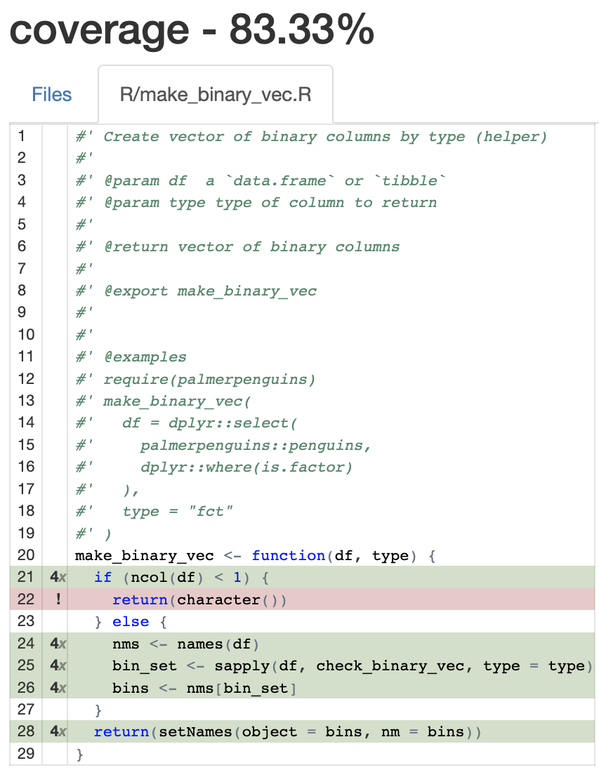
make_binary_vec()
make_binary_vec()
It’s probably not worth chasing down the remaining 17% on this function because I’ve outlined it’s primary requirements in the BDD functions:
describe("make_binary_vec() works", {
    it("logical", {
      # test code
    })
  it("integer", {
      # test code
    })
  it("character", {
      # test code
    })
  it("factor", {
      # test code
    })
})
Striving for a high percentage of coverage is a good practice, it doesn’t guarantee that the function always behaves as expected. Unit tests might execute a line of code, but still not catch a bug due to the design of the test (it’s easy to have high coverage if the unit tests are shallow and don’t check for any potential edge cases).
After developing the functions in utap, the files in the R/ folder are organized into names based on the ‘main function and its supporting helpers’:
R/
├── check_binary_vec.R
├── check_facet_vec.R
├── make_binary_vec.R
├── make_facet_vec.R
├── nin.R
├── pull_binary_cols.R
├── pull_cat_cols.R
├── pull_cols.R
├── pull_facet_cols.R
├── pull_numeric_cols.R
├── select_class.R
└── utap-package.R
The tests/testthat/ folder file names have identical names as the files in the R/ folder.
tests
├── testthat
│   ├── _snaps
│   ├── fixtures
│   │   ├── make_test_data.R
│   │   └── test_data.rds
│   ├── helper.R
│   ├── test-check_binary_vec.R
│   ├── test-check_facet_vec.R
│   ├── test-make_binary_vec.R
│   ├── test-nin.R
│   ├── test-pull_binary_cols.R
│   ├── test-pull_cat_cols.R
│   ├── test-pull_cols.R
│   ├── test-pull_facet_cols.R
│   ├── test-pull_numeric_cols.R
│   └── test-select_class.R
└── testthat.R

4 directories, 14 files
It’s common for R packages to have a general R/utils.R file that defines the ‘utility’ functions, but these files can become a catch-all for any functions that don’t have a clear home (read more here).
For example, I could stored the %nin% operator in R/utils.R (but it removes the ability to run test_coverage_active_file():
When I’ve completed a set of test files, I can use devtools::test() to check if they’re passing.
devtools::test()==> devtools::test()
ℹ Testing utap
✔ | F W S OK | Context
✔ | 23 | check_binary_vec
✔ | 3 | check_facet_vec
✔ | 4 | make_binary_vec
✔ | 3 | nin
✔ | 9 | pull_binary_cols
✔ | 4 | pull_cat_cols
✔ | 4 | pull_cols
✔ | 15 | pull_facet_cols
✔ | 2 | pull_numeric_cols
✔ | 14 | select_class
══ Results ═══════════════════
[ FAIL 0 | WARN 0 | SKIP 0 | PASS 81 ]
🎯 Your tests hit the mark 🎯The output above shows all tests are passing (and some helpful words of encouragement!). To check the code coverage for the utap package, I can run devtools::test_coverage() to view the output in the Viewer.
devtools::test_coverage()ℹ Computing test coverage for utap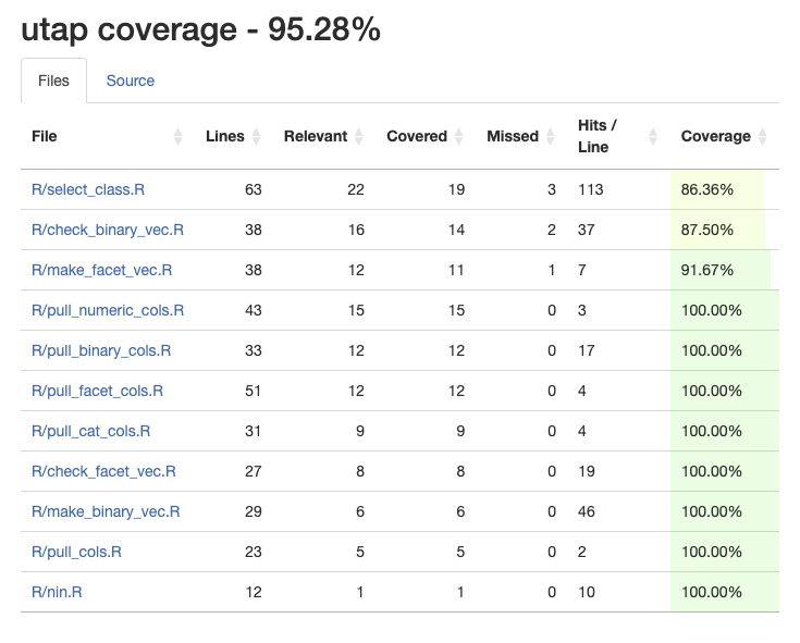
test_coverage() for entire package
devtools::test_coverage()
Clicking on any of the Files will open the Source tab and give a summary like the one above from test_coverage_active_file(). I can also use covr::package_coverage() in the Console for simpler output:
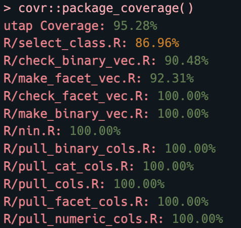
package_coverage() for entire package
covr::package_coverage()
Sometimes it’s interesting to view the relationship between function size and number of tests using the cloc package..
library(cloc)cloc stands for Count Lines of Code, and it’s a rough metric used to gauge code complexity. It’s simple, but apparently provides “just as much predictive power as more elaborate constructs like cyclomatic complexity.”source
Below is a count of the lines of code in each file in the R folder:
cloc::cloc_by_file("R")# A tibble: 13 × 6
source filename language loc blank_lines comment_lines
<chr> <chr> <chr> <int> <int> <int>
1 R "R/select_class.R" R 27 5 31
2 R "R/check_binary_vec.R" R 24 0 14
3 R "R/make_facet_vec.R" R 19 0 19
4 R "R/pull_numeric_cols.R" R 19 1 23
5 R "R/pull_binary_cols.R" R 14 0 19
6 R "R/pull_facet_cols.R" R 14 0 37
7 R "R/check_facet_vec.R" R 13 0 14
8 R "R/pull_cat_cols.R" R 13 0 18
9 R "R/make_binary_vec.R" R 10 0 19
10 R "R/pull_cols.R" R 8 0 15
11 R "R/nin.R" R 3 0 9
12 R "R/utap-package.R" R 2 0 6
13 R "" SUM 166 6 224This output also confirms the relationship between lines of code and tests.
This post has been an introduction to unit testing utility functions in a Shiny app-package. When I’m confident the utility functions are working, I’ll start adding them into modules (and testing with testServer() or shinytest2). Files names can change a lot throughout the course of developing a Shiny app-package, so it’s helpful to adopt (or create) a naming convention.9
Which particular file naming convention you choose isn’t as important as adopting a convention and implementing it.
Learn more about R packages in R Packages, 2ed↩︎
R Packages, 2ed also suggests binding test_active_file() and test_coverage_active_file() to keyboard shortcuts.↩︎
Read more about behavior-driven development in BDD in Action, 2ed↩︎
describe() and it() are discussed in the testthat documentation.↩︎
The variable names would automatically populate the choices argument for a selectInput()↩︎
testthat’s it() function is essentially identical to test_that().↩︎
Both functions are placed in R/select_class.R, and both unit tests are also in the tests/testthat/test-select_class.R file.↩︎
The fixtures name is not required, but it always make sense to keep folder names explicit.↩︎
If you’re using the golem framework to develop your shiny app-package, the utils_ and fct_ prefixes are used to define two different types of utility/helper functions. utils_ files contain ‘small helper functions and’top-level functions defining your user interface and your server function’. fct_ files contain ‘the business logic, which are potentially large functions…the backbone of the application and may not be specific to a given module’.↩︎