show/hide

# remotes::install_github("tidyverse/purrr", 
#                   force = TRUE, quiet = TRUE)
library(purrr)
library(dplyr)
library(lubridate)
library(sloop)
library(stringr)
library(snakecase)
library(waldo)

This post is going to cover the recent updates to the purrr package. The release of version 1.0.0 (and dev version v1.0.1) had some breaking changes, which I will cover below. But first, I’ll dive into some attributes of R’s functions and objects that make purrr particularly useful, and I’ll work through iteration problems I’ve encountered (and solved with purrr).

Refresher: functions and objects

If you’re like me, you’ve never been a big fan of for loops. They’re an important concept to grasp, but if you’ve ever had to debug what’s happening in multiple nested for loops, you’ve probably found yourself asking if there’s a better way to iterate.

In a functional programming language like R, it’s nice when to have functions perform a lot of the work I’d have to write into a for loop.

Generic functions & S3 objects

R’s syntax avoids explicit iteration by allowing certain generic functions to be used across different types (or objects). For example, the base plot() and summary() functions are S3 generic function:

show/hide

sloop::ftype(plot)
## [1] "S3"      "generic"
sloop::ftype(summary)
## [1] "S3"      "generic"

Which means plot() can be applied to S3 objects, like time-series (ts) and rectangular datasets (data.frame):

show/hide

sloop::otype(datasets::LakeHuron)
## [1] "S3"
class(datasets::LakeHuron)
## [1] "ts"
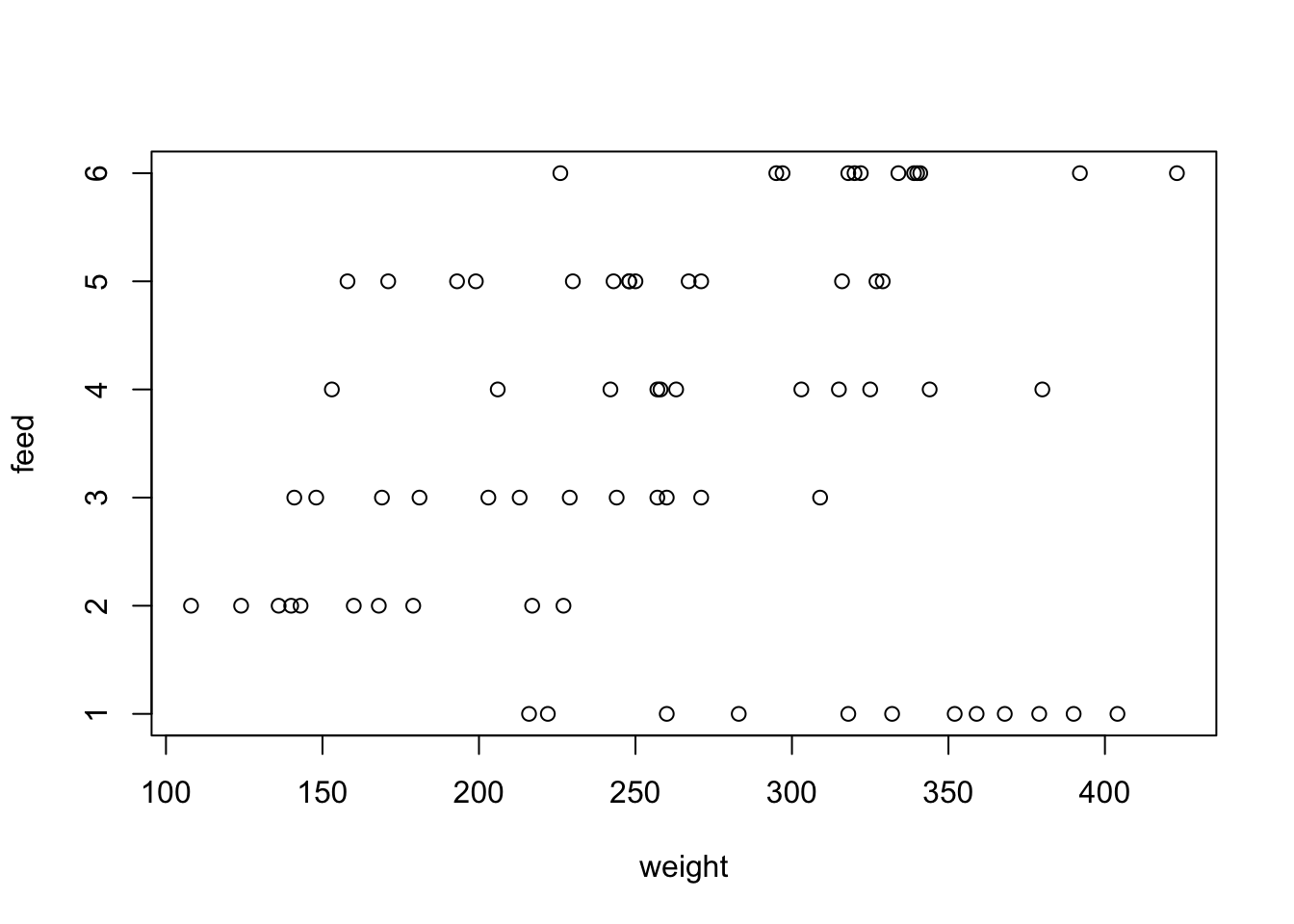
sloop::otype(datasets::chickwts)
## [1] "S3"
class(datasets::chickwts)
## [1] "data.frame"

show/hide

summary(datasets::LakeHuron)
##    Min. 1st Qu.  Median    Mean 3rd Qu.    Max. 
##   576.0   578.1   579.1   579.0   579.9   581.9
summary(datasets::chickwts)
##      weight             feed   
##  Min.   :108.0   casein   :12  
##  1st Qu.:204.5   horsebean:10  
##  Median :258.0   linseed  :12  
##  Mean   :261.3   meatmeal :11  
##  3rd Qu.:323.5   soybean  :14  
##  Max.   :423.0   sunflower:12

plot(datasets::LakeHuron)
plot(datasets::chickwts)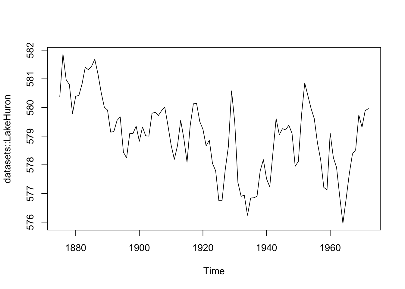

show/hide

show/hide

summary() is a particularly versatile function, because it can be used on data.frames, a single column in a data.frame, model outputs, and more.

Click Code below to view an example using summary()

show/hide

# get summary of columns ----------------------------------------------------
summary(mtcars$hp)
##    Min. 1st Qu.  Median    Mean 3rd Qu.    Max. 
##    52.0    96.5   123.0   146.7   180.0   335.0
summary(mtcars$mpg)
##    Min. 1st Qu.  Median    Mean 3rd Qu.    Max. 
##   10.40   15.43   19.20   20.09   22.80   33.90

# store model output  -------------------------------------------------------
lm_mod <- lm(formula = mpg ~ hp, data = mtcars)
lm_mod
## 
## Call:
## lm(formula = mpg ~ hp, data = mtcars)
## 
## Coefficients:
## (Intercept)           hp  
##    30.09886     -0.06823

# get summary of model output -----------------------------------------------
summary(lm_mod)
## 
## Call:
## lm(formula = mpg ~ hp, data = mtcars)
## 
## Residuals:
##     Min      1Q  Median      3Q     Max 
## -5.7121 -2.1122 -0.8854  1.5819  8.2360 
## 
## Coefficients:
##             Estimate Std. Error t value Pr(>|t|)    
## (Intercept) 30.09886    1.63392  18.421  < 2e-16 ***
## hp          -0.06823    0.01012  -6.742 1.79e-07 ***
## ---
## Signif. codes:  0 '***' 0.001 '**' 0.01 '*' 0.05 '.' 0.1 ' ' 1
## 
## Residual standard error: 3.863 on 30 degrees of freedom
## Multiple R-squared:  0.6024, Adjusted R-squared:  0.5892 
## F-statistic: 45.46 on 1 and 30 DF,  p-value: 1.788e-07

# pass the output from one S3 generic to another S3 generic -----------------
coef(summary(lm_mod))
##                Estimate Std. Error   t value     Pr(>|t|)
## (Intercept) 30.09886054  1.6339210 18.421246 6.642736e-18
## hp          -0.06822828  0.0101193 -6.742389 1.787835e-07

FP + OOP

Functional programming is complementary to object-oriented programming, which has been the dominant programming paradigm for the last several decades. - Advanced R, 2nd edition

plot() and summary() are parametric polymorphic (generic) functions, which means they have slightly different behaviors based on the objects passed into them.

As I can see, generic functions are flexible and efficient because of not having to re-define a new function for each input object–outputs from generic functions will automatically change (in part) depending on the structure of the object provided to them.

The relationship between functions and objects is what makes purrr (and other tools for iteration) extremely helpful for solving iteration problems we commonly encounter when working with data. Similar to generic functions, these functions allow us to express iterative behavior using a complete and consistent set of tools.

Iteration problems

In programming, iteration refers to defining an input and applying an operation over every part of it. Some examples of problems that iteration can solve include:

You have a list of objects and you’d like to apply a function (or a series of functions) over the elements in the list
You have a folder full of files you’d like to rename or copy to a new directory
You’d like to download a collection of files from separate URLS
You have several years of data, and each year is contained in separate file. You’d like to read these data into R, combine them into a single dataset
You have a non-rectangular (i.e., list) of datasets you’d like to split into individual data.frames, then export these into separate file paths.

These are all problems I’ve personally encountered that required a variety of iteration tools to tackle. I’ll start with the first example because the principles remain the same (regardless of the size/scope of the problem):

The `for` loop

for loops are ubiquitous in programming, and (for the most part) they describe the types of problems they’re solving:

“for each item in object, do operation”

I have a list (my_list), with items in various cases:

show/hide

my_list
## $words
## [1] "MOvE"     "tHURsDAy" "SISter"   "jOiN"     "lASt"    
## 
## $sentences
## [1] "THe tHefT oF the Pearl PIN WaS kePT SEcrEt."    
## [2] "iT snOWed, RAINEd, AND HaIled ThE samE MOrNiNG."
## [3] "IT caUght iTs HINd pAw in a ruSTY tRaP."        
## 
## $letters
##  [1] "W" "G" "T" "q" "X" "S" "O" "P" "u" "L"

If I try to use the tolower() on my_list, it returns a vector.

show/hide

tolower(my_list) |> str()
##  chr [1:3] "c(\"move\", \"thursday\", \"sister\", \"join\", \"last\")" ...

How can I apply the tolower() function to each item in my_list, and return the original object type? I’ll use my_list and tolower() to demonstrate how I was taught to write for loops:

First: define the sequence, ‘for [item] in [items in object]’

In this case, x is the abstracted [item] taking on the values returned by seq_along(my_list) (the [items in object])

show/hide

seq_along(my_list)
## [1] 1 2 3
# take single value of 'x'
seq_along(my_list)[1]
## [1] 1
# use this to get 'items in object'
my_list[[seq_along(my_list)[1]]]
## [1] "MOvE"     "tHURsDAy" "SISter"   "jOiN"     "lASt"

Second: write the operations the for loop will perform per iteration (i.e. the first iteration is x = tolower(my_list[[1]]); the second iteration is x = tolower(my_list[[2]]); etc.)
- Test this with a few values if you like
show/hide
tolower(my_list[[2]]) ## [1] "the theft of the pearl pin was kept secret." ## [2] "it snowed, rained, and hailed the same morning." ## [3] "it caught its hind paw in a rusty trap."

Third: define an (optional) object to capture the results of the loop (lc_list), and make sure it’s the correct size

Two methods for creating empty lists

show/hide

vector(mode = "list", length = 3)
## [[1]]
## NULL
## 
## [[2]]
## NULL
## 
## [[3]]
## NULL
list(NULL, NULL, NULL)
## [[1]]
## NULL
## 
## [[2]]
## NULL
## 
## [[3]]
## NULL

Finally, we put it all together in a for loop

show/hide

# define capture object
lc_list <- vector(mode = "list", length = 3)
# write sequence
for (x in seq_along(my_list)) {        
  # write operations/capture in object
  lc_list[[x]] <- tolower(my_list[[x]])
  # clean up container
  names(lc_list) <- c("words", "sentences", "letters")
}
lc_list
## $words
## [1] "move"     "thursday" "sister"   "join"     "last"    
## 
## $sentences
## [1] "the theft of the pearl pin was kept secret."    
## [2] "it snowed, rained, and hailed the same morning."
## [3] "it caught its hind paw in a rusty trap."        
## 
## $letters
##  [1] "w" "g" "t" "q" "x" "s" "o" "p" "u" "l"

This was a simple example, but it demonstrates the basic components in a for loop:

The sequence to index
- for (x in seq_along(my_list))
The operations to iterate
- tolower(my_list[[x]])
The object to capture the results
- lc_list <- vector(mode = "list", length = 3) and
- lc_list[[x]]

Base R

base R has the _apply family of functions (apply(), lapply(), sapply(), vapply(), etc.) that remove a lot of the ‘book keeping’ code we had to write in the for loop.

`lapply()`

Sticking with the my_list and tolower() example, the apply function I want is lapply() (pronounced ‘l-apply’), and the l stands for list.

lapply() has only two required arguments:

X the object we want to iterate over
FUN being the function we want iterated

show/hide

lapply(X = my_list, FUN = tolower)
## $words
## [1] "move"     "thursday" "sister"   "join"     "last"    
## 
## $sentences
## [1] "the theft of the pearl pin was kept secret."    
## [2] "it snowed, rained, and hailed the same morning."
## [3] "it caught its hind paw in a rusty trap."        
## 
## $letters
##  [1] "w" "g" "t" "q" "x" "s" "o" "p" "u" "l"

`sapply()`

sapply() attempts to simplify the result depending on the X argument. If X is a list containing vectors where every element has the same length (and it’s greater than 1), then sapply() returns a matrix:

show/hide

str(my_list[1])
## List of 1
##  $ words: chr [1:5] "MOvE" "tHURsDAy" "SISter" "jOiN" ...
sapply(X = my_list[1], FUN = tolower)
##      words     
## [1,] "move"    
## [2,] "thursday"
## [3,] "sister"  
## [4,] "join"    
## [5,] "last"

If a vector is passed to X where every element is length 1, then a vector is returned:

show/hide

str(my_list[[1]])
##  chr [1:5] "MOvE" "tHURsDAy" "SISter" "jOiN" "lASt"
sapply(X = my_list[[1]], FUN = tolower) 
##       MOvE   tHURsDAy     SISter       jOiN       lASt 
##     "move" "thursday"   "sister"     "join"     "last"

Finally, if X is a list where elements have a length greater than 1, then a list is returned (making it identical to lapply()

show/hide

waldo::compare(
  x = sapply(X = my_list, FUN = tolower), 
  y = lapply(X = my_list, FUN = tolower)
)
## ✔ No differences

This is because sapply is a wrapper around lapply, but has simplify and USE.NAMES set to FALSE (see what happens below when I change them to TRUE)

show/hide

waldo::compare(
  
  x = lapply(X = my_list[[1]], FUN = tolower), 
  
  y = sapply(X = my_list[[1]], FUN = tolower, 
              simplify = TRUE, USE.NAMES = TRUE)
  
  )
## `old` is a list
## `new` is a character vector ('move', 'thursday', 'sister', 'join', 'last')

Anonmymous functions

The FUN argument can also take anonymous (undefined) functions. For example, if I wanted to access the second elements in my_list, I could pass an anonymous function the FUN (with the index):

show/hide

lapply(X = my_list, FUN = function(x) x[[2]])
## $words
## [1] "tHURsDAy"
## 
## $sentences
## [1] "iT snOWed, RAINEd, AND HaIled ThE samE MOrNiNG."
## 
## $letters
## [1] "G"

`vapply()`

Finally vapply() is unique in that it always simplifies the returned output. If we repeat the example above, we see the returned value is character vector:

show/hide

vapply(X = my_list, 
  FUN = function(x) x[[2]], 
  FUN.VALUE = character(1))
##                                             words 
##                                        "tHURsDAy" 
##                                         sentences 
## "iT snOWed, RAINEd, AND HaIled ThE samE MOrNiNG." 
##                                           letters 
##                                               "G"

The apply functions get us much further than writing for loops because we can 1) iterate over vectors and lists, 2) control the output objects, and 3) write less code. Unlike generic functions, apply functions are designed to work with specific object types, and return values depending on these objects.

One downside of apply functions is they don’t play well with data.frames or tibbles. However, we can control their return values (and manually supply these to tibble::tibble() or data.frame()

show/hide

tibble::tibble(
  words = vapply(X = my_list[[1]][1:3], 
                FUN = `[`, 
                FUN.VALUE = character(1)),
  sentences = vapply(X = my_list[[2]][1:3], 
                    FUN = `[`, 
                    FUN.VALUE = character(1)),
  letters = vapply(X = my_list[[3]][1:3], 
                  FUN = `[`, 
                  FUN.VALUE = character(1)))

Another downside of the apply functions is they’re not very uniform. Each function has slight variations in their arguments and rules for return values. This is where purrr comes in…

`purrr`

If you’re new to purrr, a great way to start using it’s functions is with a recipe covered in Charlotte Wickham’s tutorial

Do it for one element
Turn it into a recipe
Use purrr::map() to do it for all elements

I’ll work through these three steps below using my_list and tolower()

1. Do it for one element

The goal with the first step is to get a minimal working example with a single element from the object I want to iterate over (with the function I want to iterate with).

For this example, I need to subset my_list for a single element at position [[1]], [[2]], or [[3]] (or using one of the vector names).

I’ll then pass this element to tolower() and make sure it’s the desired behavior:

# subset an element from the list
? <- my_list[[?]]
# apply a function to extracted element
tolower(?)

? <- my_list[[?]] = subset element from the list (my_list)
tolower(?) = apply operation (i.e., function) to extracted element.

show/hide

my_words <- my_list[['words']]
tolower(my_words)
## [1] "move"     "thursday" "sister"   "join"     "last"

Now that I have a working example for one element, in the next step I’ll abstract these parts into the function arguments.

2. Turn it into a recipe

A standard purrr recipe defines .x (the object) and .f (the function), followed by any additional function arguments.

.x = a list or atomic vector
.f = the function we want to apply over every element in .x

.x = my_list, .f = tolower

3. `map()` it across all elements

In purrr::map(), the .x argument is the object (list or atomic vector) I want to iterate over, and .f is the function (i.e., operation) I want applied to every element of .x

If I want to convert the case of every element in my_list to lowercase with tolower() I would use the following standard purrr::map() format:

show/hide

purrr::map(.x = my_list, .f = tolower)
## $words
## [1] "move"     "thursday" "sister"   "join"     "last"    
## 
## $sentences
## [1] "the theft of the pearl pin was kept secret."    
## [2] "it snowed, rained, and hailed the same morning."
## [3] "it caught its hind paw in a rusty trap."        
## 
## $letters
##  [1] "w" "g" "t" "q" "x" "s" "o" "p" "u" "l"

And there you have it! map() is the core function and workhorse of the purrr package. It’s important to note that purrr::map() always returns a list, regardless of the object supplied to .x.

Version 1.0.0 updates

Now I’ll cover some of the updates in purrr 1.0.0. I’ll be using mixed_list, a list with five different types of vectors.

show/hide

mixed_list
## $booleans
## [1]  TRUE FALSE  TRUE FALSE
## 
## $integers
## [1]  4  7  8  1 10
## 
## $doubles
## [1] 2.909 2.938 2.853 2.755 2.990
## 
## $strings
## [1] "second" "commit" "red"    "except" "fire"  
## 
## $dates
## [1] "2023-12-06" "2023-10-27" "2023-09-07"

`map()` updates

As noted above, by default purrr::map() returns a list. If I’d like to return a vector, I can use one of the map_ variations (there’s one for each vector type).

By mapping the is.<type>() functions the elements in mixed_list, I can test which elements in mixed_list return TRUE:

map_lgl(): returns a logical vector

show/hide

mixed_list |> purrr::map_lgl(\(x) is.logical(x))

booleans integers  doubles  strings    dates 
    TRUE    FALSE    FALSE    FALSE    FALSE

map_int(): returns an integer vector

show/hide

mixed_list |> purrr::map_int(\(x) is.integer(x))

booleans integers  doubles  strings    dates 
       0        1        0        0        0

map_dbl(): returns a double vector

show/hide

mixed_list |> purrr::map_dbl(\(x) is.double(x))

booleans integers  doubles  strings    dates 
       0        0        1        0        1

map_chr(): returns a character vector

show/hide

mixed_list |> purrr::map_chr(\(x) is.character(x))

Warning: Automatic coercion from logical to character was deprecated in purrr 1.0.0.
ℹ Please use an explicit call to `as.character()` within `map_chr()` instead.

booleans integers  doubles  strings    dates 
 "FALSE"  "FALSE"  "FALSE"   "TRUE"  "FALSE"

When we test for characters in mixed_list, we see the following warning:

Warning: Automatic coercion from logical to character was deprecated in purrr 1.0.0. Please use an explicit call to as.character() within map_chr() instead

As we can see from the output above, the logical return values from is.character() are coerced to characters (this behavior is now deprecated).

`map_vec()`

However, the previous purrr::map_raw() function has been replaced with purrr::map_vec(), which “simplifies to the common type of the output.” I’ll demonstrate below with the characters in mixed_list:

show/hide

mixed_list |> purrr::map_vec(\(x) is.character(x))
## booleans integers  doubles  strings    dates 
##    FALSE    FALSE    FALSE     TRUE    FALSE

Notice the difference in output? The results are the same as above, but output is not commented (##). The same is true when I test the dates in mixed_list using lubridate::is.Date():

show/hide

mixed_list |> purrr::map_vec(\(x) lubridate::is.Date(x))
## booleans integers  doubles  strings    dates 
##    FALSE    FALSE    FALSE    FALSE     TRUE

Anonymous functions

R introduced the shorthand anonymous function syntax in version 4.1.0:

“\(x) x + 1 is parsed as function(x) x + 1.”

Below is a comparison of an anonymous (unnamed) function and the updated shorthand syntax:

Standard anonymous function

show/hide

(function(x) tolower(x))("pIrAtES Ship")
## [1] "pirates ship"

The updated anonymous syntax is below:

show/hide

(\(x) tolower(x))("pIrAtES Ship")
## [1] "pirates ship"

Writing the code above using an anonymous function would look like this:

show/hide

my_list |> purrr::map(\(x) tolower(x))
## $words
## [1] "move"     "thursday" "sister"   "join"     "last"    
## 
## $sentences
## [1] "the theft of the pearl pin was kept secret."    
## [2] "it snowed, rained, and hailed the same morning."
## [3] "it caught its hind paw in a rusty trap."        
## 
## $letters
##  [1] "w" "g" "t" "q" "x" "s" "o" "p" "u" "l"

Anonymous functions make it easier to understand which arguments belong to which function and will tend to yield better error messages.

I’ll confirm the outputs from both methods are identical using waldo::compare():

show/hide

waldo::compare(
  x = purrr::map(.x = my_list, .f = tolower), 
  y = my_list |> purrr::map(\(x) tolower(x)))
## ✔ No differences

The formula (~ .x + 1)

Prior to purrr v1.0.0, I could also use the formula syntax, but now it’s “only recommended if you require backward compatibility with older versions of R.” I’ll cover the formula syntax briefly because you’re likely to encounter it.

The formula syntax is typically used with pipes, so the contents of purrr::map() become the right-hand side of the formula, with the function we want to iterate (<FUNCTION>) and a placeholder (.x) in the appropriate argument.

<OBJECT> |> purrr::map(~ <FUNCTION>(.x))

For the example above, my_list is ‘piped’ to purrr::map(), where the formula maps the tolower() function (using the .x placeholder).

# written as normal expression
 my_list |> purrr::map(~ tolower(.x))

Jenny Bryan offers a great description on her purrr tutorial,

“[formula syntax] should start with the ~ symbol and then look like a typical top-level expression, as you might write in a script. Use .x to refer to the input, i.e. an individual element of the primary vector or list.”

I can double-check to see that the output from two variations are identical using waldo::compare().

show/hide

waldo::compare(
  x = my_list |> purrr::map(\(x) tolower(x)), 
  y = my_list |> purrr::map(~ tolower(.x)))
## ✔ No differences

Worked Examples

In this section, I’ll be working through some of the uses I’ve for purrr’s functions. I’ve tried to choose tasks that are common across most projects so my code can be easily copied and adapted.

Downloading files

You’d like to download a collection of files from separate URLS

I have a collection of 30 .csv files from Doing Data Science by Cathy O’Neil and Rachel Schutt (O’Reilly Media) in a GitHub repo. Let’s assume I want to download one week of these files into my RStudio session (without downloading the repo).

I’ll navigate to the raw url for the first data file (nyt1.csv), then paste this into a character vector:

show/hide

nyt_url <- "https://raw.githubusercontent.com/mjfrigaard/dds-data/main/nyt1.csv"

Knowing that all of the files on GitHub with have a similar sheme and domain, I can use nyt_url to generate urls for each of the 7 files.

First I get the folder of the files on GitHub with fs::path_dir()

show/hide

# create file urls 
nyt_dir_url <- fs::path_dir(nyt_url)
nyt_dir_url

[1] "https:/raw.githubusercontent.com/mjfrigaard/dds-data/main"

I create a vector with the 7 file names

show/hide

# create file names for 7th through 13th
nyt_file_nms <- paste0("nyt", 7:13, ".csv")
nyt_file_nms

[1] "nyt7.csv"  "nyt8.csv"  "nyt9.csv"  "nyt10.csv" "nyt11.csv" "nyt12.csv"
[7] "nyt13.csv"

I combine the directory portion of the url with file name in nyt_file_urls

show/hide

# combine
nyt_file_urls <- paste(nyt_dir_url, nyt_file_nms, sep = "/")
nyt_file_urls

[1] "https:/raw.githubusercontent.com/mjfrigaard/dds-data/main/nyt7.csv" 
[2] "https:/raw.githubusercontent.com/mjfrigaard/dds-data/main/nyt8.csv" 
[3] "https:/raw.githubusercontent.com/mjfrigaard/dds-data/main/nyt9.csv" 
[4] "https:/raw.githubusercontent.com/mjfrigaard/dds-data/main/nyt10.csv"
[5] "https:/raw.githubusercontent.com/mjfrigaard/dds-data/main/nyt11.csv"
[6] "https:/raw.githubusercontent.com/mjfrigaard/dds-data/main/nyt12.csv"
[7] "https:/raw.githubusercontent.com/mjfrigaard/dds-data/main/nyt13.csv"

I’ll need another vector of destination file names on my local machine, which I can do by combining the file names (nyt_file_nms) with the local destination folder (dds-nyt).

show/hide

nyt_local_pths <- paste("dds-nyt", nyt_file_nms, sep = "/")
nyt_local_pths

[1] "dds-nyt/nyt7.csv"  "dds-nyt/nyt8.csv"  "dds-nyt/nyt9.csv" 
[4] "dds-nyt/nyt10.csv" "dds-nyt/nyt11.csv" "dds-nyt/nyt12.csv"
[7] "dds-nyt/nyt13.csv"

After creating the destination folder, I’ll use the download.file() function to test downloading a single .csv files into my local folder (dds-nyt/). download.file() has a progress bar which tells me if the file downloaded successfully.

show/hide

# do it for one
fs::dir_create("dds-nyt")
download.file(url = nyt_file_urls[1], destfile = nyt_local_pths[1])

trying URL 'https:/raw.githubusercontent.com/mjfrigaard/dds-data/main/nyt1.csv'
Content type 'text/plain; charset=utf-8' length 4920381 bytes (4.7 MB)
==================================================
downloaded 4.7 MB

download.file() takes two inputs (url and destfile), which changes the recipe a bit, because I need a purrr function with the following:

.x the input vector of existing url paths
.y the output vector of destination file paths
Additional arguments passed from download.file() (like quiet = TRUE)

In this case, I don’t need purrr to return value–I just need the purrr function to iterate over the items and write them to the new location.

walk() is ideal for this circumstance:

“walk() returns the input .x (invisibly)” and “The return value of .f() is ignored”

What do ‘return .x invisibly’ and ‘the side-effect of .f’ mean?

Return invisibly

The previous purrr functions I covered varied in the kinds of values they returned (lists vs. vectors), but for some operations I won’t need a return value. If I’m ever curious about whether I should be using map() or walk(), I’ll ask myself, “would it make sense to assign the output from this function to an object?”

If the answer is no, then I probably need to be thinking walk() instead of map()

Side-effects

In the help documentation walk()’s description states, “calls .f for its side-effect”, which can be generally interpreted as, “there’s nothing to assign the output from that function to.”

`purrr` progress bars

I’ll use walk2() below and add .progress = TRUE to view the purrr progress bar (and quiet = TRUE to silence the download.file() progress bar).

show/hide

walk2(.x = nyt_file_urls, .y = nyt_local_pths, .f =  download.file, 
      .progress = TRUE, quiet = TRUE)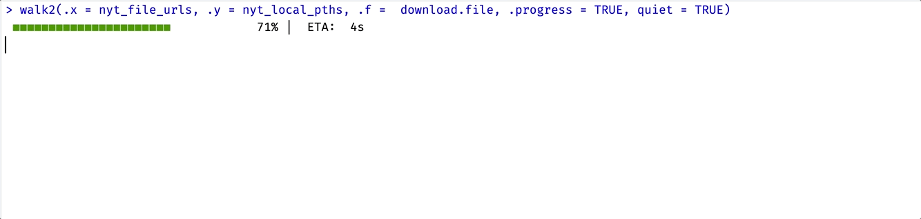

I can confirm the download using fs::dir_tree()

show/hide

fs::dir_tree("dds-nyt")
## dds-nyt
## ├── nyt10.csv
## ├── nyt11.csv
## ├── nyt12.csv
## ├── nyt13.csv
## ├── nyt7.csv
## ├── nyt8.csv
## └── nyt9.csv

Copying a directory of files

You have a folder of files you’d like to rename or copy to a new directory

The collection of 7 .csv files from Doing Data Science by Cathy O’Neil and Rachel Schutt (O’Reilly Media) are now in the dds-nyt/ folder.

As with any project, I don’t want to alter the raw data, so I’m going to copy these files into dds-nyt-raw/ and dds-nyt-processed/. I also want the processed file names to have a date stamp prefix.

show/hide

file_pths <- list.files("dds-nyt", full.names = TRUE, pattern = ".csv$")
file_pths
## [1] "dds-nyt/nyt10.csv" "dds-nyt/nyt11.csv" "dds-nyt/nyt12.csv"
## [4] "dds-nyt/nyt13.csv" "dds-nyt/nyt7.csv"  "dds-nyt/nyt8.csv" 
## [7] "dds-nyt/nyt9.csv"

I’ll start with the raw data folder. I need to create a vector of the new raw file paths and names: raw_file_pths (the raw data paths will have the original file names)

show/hide

# do it for one
gsub(pattern = "^dds-nyt",
  replacement = "dds-nyt/raw",
  x = file_pths[1])
## [1] "dds-nyt/raw/nyt10.csv"

# write the recipe
file_pths |> purrr::map_chr(\(x) gsub(x, 
                                pattern = "^dds-nyt", 
                                replacement = "dds-nyt/raw")) |> head()
## [1] "dds-nyt/raw/nyt10.csv" "dds-nyt/raw/nyt11.csv" "dds-nyt/raw/nyt12.csv"
## [4] "dds-nyt/raw/nyt13.csv" "dds-nyt/raw/nyt7.csv"  "dds-nyt/raw/nyt8.csv"

# map it across all
raw_file_pths <- file_pths |> 
                  purrr::map_chr(\(x) gsub(x, 
                                        pattern = "^dds-nyt", 
                                        replacement = "dds-nyt/raw"))

Before copying the files, I need to create the destination folder for the raw data (dds-nyt/raw). Then, I’ll make sure I can copy the first element from file_pths into the path in the first element of raw_file_pths:

show/hide

fs::dir_create("dds-nyt/raw")
# do it for one
fs::file_copy(
  path = file_pths[1], 
  new_path = raw_file_pths[1], 
  overwrite = TRUE)
fs::dir_tree("dds-nyt/raw", type = "any")
## dds-nyt/raw
## └── nyt10.csv

I can see this is working, so I can use purrr::walk2() to move all the files from dds-nyt/ to dds-nyt/raw/

show/hide

purrr::walk2(.x = file_pths, .y = raw_file_pths, .f = fs::file_copy, 
      .progress = TRUE, overwrite = TRUE)
fs::dir_tree("dds-nyt/raw", type = "any")
## dds-nyt/raw
## ├── nyt10.csv
## ├── nyt11.csv
## ├── nyt12.csv
## ├── nyt13.csv
## ├── nyt7.csv
## ├── nyt8.csv
## └── nyt9.csv

Now that I’ve copied the files into their respective folders, I’ll need to remove the files from their original location in the parent dds-nyt folder.

Fortunately, I have a vector of these files in file_pths, and I can test removal with fs::file_delete():

show/hide

fs::file_delete(file_pths[1])

Great! Now that I know this will work, I’ll use walk() because I want .x returned invisibly and the side-effect of .f.

But I’ve also deleted the first element in file_pths, so when fs::file_delete() goes looking for that file, it will find nothing and returned an error.

show/hide

Error in `map()`:
ℹ In index: 1.
Caused by error:
! [ENOENT] Failed to remove 'dds-nyt/nyt10.csv': no such file or directory

I can protect against this by supplying the output from list.files() directly to purrr::walk2(), but include a pattern so it only matches the .csv files.

show/hide

purrr:::walk(
  # list CURRENT files 
    .x = list.files(
      path = "dds-nyt",
      pattern = ".csv$",
      full.names = TRUE),
    # map function
    .f = fs::file_delete)

And confirm the new folder contents and structure

show/hide

fs::dir_tree("dds-nyt", type = "any", recurse = TRUE)
## dds-nyt
## └── raw
##     ├── nyt10.csv
##     ├── nyt11.csv
##     ├── nyt12.csv
##     ├── nyt13.csv
##     ├── nyt7.csv
##     ├── nyt8.csv
##     └── nyt9.csv

Import multiple datasets

You have several days of data, and each day is contained in separate file. You’d like to read these data into R, and combine them into a single dataset

Now that I have separate raw and processed folders, I can import the NYT data into R. Below I’ve imported a single file from the raw data folder to examine it’s contents:

show/hide

nyt1 <- vroom::vroom(file = raw_file_pths[1],
  delim = ",", 
  show_col_types = FALSE)
str(nyt1)
## spc_tbl_ [452,766 × 5] (S3: spec_tbl_df/tbl_df/tbl/data.frame)
##  $ Age        : num [1:452766] 59 0 19 44 30 33 41 41 0 23 ...
##  $ Gender     : num [1:452766] 1 0 0 1 1 1 0 0 0 1 ...
##  $ Impressions: num [1:452766] 4 7 5 5 4 3 1 3 9 1 ...
##  $ Clicks     : num [1:452766] 0 1 0 0 0 0 0 0 1 0 ...
##  $ Signed_In  : num [1:452766] 1 0 1 1 1 1 1 1 0 1 ...
##  - attr(*, "spec")=
##   .. cols(
##   ..   Age = col_double(),
##   ..   Gender = col_double(),
##   ..   Impressions = col_double(),
##   ..   Clicks = col_double(),
##   ..   Signed_In = col_double(),
##   ..   .delim = ","
##   .. )
##  - attr(*, "problems")=<externalptr>

Each nyt file contains daily ads shown and clicks recorded on the New York Times home page. The rows represent users, and the variables are: Age, Gender (0 = female, 1 = male), Impressions (number impressions), Clicks (number clicks), and a binary indicator for signed in or not Signed_in.

I’ll add some hypothetical wrangling steps to make this example more realistic.

Create age_group, an ordered factor which contains six levels of Age (“<18”, “18-24”, “25-34”, “35-44”, “45-54”, “55-64”, and “65+”)
Create ctr_rate or click-through rate, calculated as the number of clicks / the number of impressions. Round it to 3 digits.
Create female, a factor version of Gender, where when Gender = 0, then female = "yes", and when Gender = 1, then female = "no"
Create signed_in, a factor variable with levels "no" and "yes" from the Signed_In = 0 and 1

I’ve bundled all of these steps into a function (nyt_data_processing()) that I can pass each dataset through:

show/hide

nyt_data_processing <- function(nyt_csv) {
  orig_nms <- c("Age", "Gender", "Impressions", "Clicks", "Signed_In")
  nyt_nms <- names(nyt_csv)
  if (isFALSE(identical(x = orig_nms, y = nyt_nms))) {
    cli::cli_abort("these data don't have the correct columns!")
  } else {
    nyt_proc <- nyt_csv |>
      dplyr::mutate(
        # create age_group variable
        age_group = case_when(
          Age < 18 ~ "<18",
          Age >= 18 & Age < 25 ~ "18-24",
          Age >= 25 & Age < 35 ~ "25-34",
          Age >= 35 & Age < 45 ~ "35-44",
          Age >= 45 & Age < 55 ~ "45-54",
          Age >= 55 & Age < 65 ~ "55-64",
          Age >= 65 ~ "65+"
        ),
        # factor age_group (ordered)
        age_group = factor(age_group,
          levels = c(
            "<18", "18-24", "25-34",
            "35-44", "45-54", "55-64", "65+"
          ),
          ordered = TRUE
        ),
        # create CTR variable
        ctr_rate = round(x = Clicks / Impressions, digits = 3),
        # create new Female variable
        female = case_when(
          Gender == 0 ~ "yes",
          Gender == 1 ~ "no",
          TRUE ~ NA_character_
        ),
        # factor female (un-ordered)
        female = factor(female,
          levels = c("no", "yes")
        ),
        Signed_In = case_when(
          Signed_In == 0 ~ "no", 
          Signed_In == 1 ~ "yes", 
          TRUE ~ NA_character_),
        # factor Signed_In (un-ordered) 
        Signed_In = factor(Signed_In, levels = c("no", "yes"))) |>
      # format columns
      janitor::clean_names()
  }
  return(nyt_proc)
}

I’ll do some quick checks to make sure it only works with the raw data columns:

show/hide

nyt1_proc <- nyt_data_processing(nyt1)
str(nyt1_proc)
## spc_tbl_ [452,766 × 8] (S3: spec_tbl_df/tbl_df/tbl/data.frame)
##  $ age        : num [1:452766] 59 0 19 44 30 33 41 41 0 23 ...
##  $ gender     : num [1:452766] 1 0 0 1 1 1 0 0 0 1 ...
##  $ impressions: num [1:452766] 4 7 5 5 4 3 1 3 9 1 ...
##  $ clicks     : num [1:452766] 0 1 0 0 0 0 0 0 1 0 ...
##  $ signed_in  : Factor w/ 2 levels "no","yes": 2 1 2 2 2 2 2 2 1 2 ...
##  $ age_group  : Ord.factor w/ 7 levels "<18"<"18-24"<..: 6 1 2 4 3 3 4 4 1 2 ...
##  $ ctr_rate   : num [1:452766] 0 0.143 0 0 0 0 0 0 0.111 0 ...
##  $ female     : Factor w/ 2 levels "no","yes": 1 2 2 1 1 1 2 2 2 1 ...
##  - attr(*, "spec")=
##   .. cols(
##   ..   Age = col_double(),
##   ..   Gender = col_double(),
##   ..   Impressions = col_double(),
##   ..   Clicks = col_double(),
##   ..   Signed_In = col_double(),
##   ..   .delim = ","
##   .. )
##  - attr(*, "problems")=<externalptr>

I’ll run nyt_data_processing() against a processed data file (nyt1_proc)

show/hide

nyt_data_processing(nyt1_proc)
## Error in `nyt_data_processing()`:
## ! these data don't have the correct columns!

Now I’m ready to write the import step. First I’ll store the raw file paths in raw_data_pths

show/hide

raw_data_pths <- list.files(path = "dds-nyt/raw", pattern = ".csv$", full.names = TRUE)

We’ll test purrr::map() and vroom::vroom() to import the .csv files in raw_data_pths into a list. I also add utils::head() and dplyr::glimpse() to limit the output.

show/hide

raw_data_pths |> 
  # import
  purrr::map(
    vroom::vroom, 
        delim = ",", show_col_types = FALSE) |> 
  utils::head(2) |> 
  dplyr::glimpse()
## List of 2
##  $ : spc_tbl_ [452,766 × 5] (S3: spec_tbl_df/tbl_df/tbl/data.frame)
##   ..$ Age        : num [1:452766] 59 0 19 44 30 33 41 41 0 23 ...
##   ..$ Gender     : num [1:452766] 1 0 0 1 1 1 0 0 0 1 ...
##   ..$ Impressions: num [1:452766] 4 7 5 5 4 3 1 3 9 1 ...
##   ..$ Clicks     : num [1:452766] 0 1 0 0 0 0 0 0 1 0 ...
##   ..$ Signed_In  : num [1:452766] 1 0 1 1 1 1 1 1 0 1 ...
##   ..- attr(*, "spec")=
##   .. .. cols(
##   .. ..   Age = col_double(),
##   .. ..   Gender = col_double(),
##   .. ..   Impressions = col_double(),
##   .. ..   Clicks = col_double(),
##   .. ..   Signed_In = col_double(),
##   .. ..   .delim = ","
##   .. .. )
##   ..- attr(*, "problems")=<externalptr> 
##  $ : spc_tbl_ [478,066 × 5] (S3: spec_tbl_df/tbl_df/tbl/data.frame)
##   ..$ Age        : num [1:478066] 28 51 29 20 19 0 58 42 35 44 ...
##   ..$ Gender     : num [1:478066] 1 0 1 1 0 0 0 0 1 0 ...
##   ..$ Impressions: num [1:478066] 8 5 2 4 5 3 5 6 8 4 ...
##   ..$ Clicks     : num [1:478066] 0 0 0 0 0 1 1 0 0 0 ...
##   ..$ Signed_In  : num [1:478066] 1 1 1 1 1 0 1 1 1 1 ...
##   ..- attr(*, "spec")=
##   .. .. cols(
##   .. ..   Age = col_double(),
##   .. ..   Gender = col_double(),
##   .. ..   Impressions = col_double(),
##   .. ..   Clicks = col_double(),
##   .. ..   Signed_In = col_double(),
##   .. ..   .delim = ","
##   .. .. )
##   ..- attr(*, "problems")=<externalptr>

This returns a list, but you may have noticed I don’t have a great way for keeping track of the data files in the list–this is where purrr::set_names() comes in handy.

purrr::set_names() works a lot like names(), but purrr::set_names() will automatically set the names of x to as.character(x) if no names are provided to nm. See below:

show/hide

raw_data_pths |> purrr::set_names()
##   dds-nyt/raw/nyt10.csv   dds-nyt/raw/nyt11.csv   dds-nyt/raw/nyt12.csv 
## "dds-nyt/raw/nyt10.csv" "dds-nyt/raw/nyt11.csv" "dds-nyt/raw/nyt12.csv" 
##   dds-nyt/raw/nyt13.csv    dds-nyt/raw/nyt7.csv    dds-nyt/raw/nyt8.csv 
## "dds-nyt/raw/nyt13.csv"  "dds-nyt/raw/nyt7.csv"  "dds-nyt/raw/nyt8.csv" 
##    dds-nyt/raw/nyt9.csv 
##  "dds-nyt/raw/nyt9.csv"

Now the imported file will have their file path and name associated with the dataset:

show/hide

raw_data_pths |> 
  # names 
  purrr::set_names() |> 
  # import  
    purrr::map(
      vroom::vroom, 
          delim = ",", show_col_types = FALSE) |> 
  utils::head(2) |> 
  dplyr::glimpse()
## List of 2
##  $ dds-nyt/raw/nyt10.csv: spc_tbl_ [452,766 × 5] (S3: spec_tbl_df/tbl_df/tbl/data.frame)
##   ..$ Age        : num [1:452766] 59 0 19 44 30 33 41 41 0 23 ...
##   ..$ Gender     : num [1:452766] 1 0 0 1 1 1 0 0 0 1 ...
##   ..$ Impressions: num [1:452766] 4 7 5 5 4 3 1 3 9 1 ...
##   ..$ Clicks     : num [1:452766] 0 1 0 0 0 0 0 0 1 0 ...
##   ..$ Signed_In  : num [1:452766] 1 0 1 1 1 1 1 1 0 1 ...
##   ..- attr(*, "spec")=
##   .. .. cols(
##   .. ..   Age = col_double(),
##   .. ..   Gender = col_double(),
##   .. ..   Impressions = col_double(),
##   .. ..   Clicks = col_double(),
##   .. ..   Signed_In = col_double(),
##   .. ..   .delim = ","
##   .. .. )
##   ..- attr(*, "problems")=<externalptr> 
##  $ dds-nyt/raw/nyt11.csv: spc_tbl_ [478,066 × 5] (S3: spec_tbl_df/tbl_df/tbl/data.frame)
##   ..$ Age        : num [1:478066] 28 51 29 20 19 0 58 42 35 44 ...
##   ..$ Gender     : num [1:478066] 1 0 1 1 0 0 0 0 1 0 ...
##   ..$ Impressions: num [1:478066] 8 5 2 4 5 3 5 6 8 4 ...
##   ..$ Clicks     : num [1:478066] 0 0 0 0 0 1 1 0 0 0 ...
##   ..$ Signed_In  : num [1:478066] 1 1 1 1 1 0 1 1 1 1 ...
##   ..- attr(*, "spec")=
##   .. .. cols(
##   .. ..   Age = col_double(),
##   .. ..   Gender = col_double(),
##   .. ..   Impressions = col_double(),
##   .. ..   Clicks = col_double(),
##   .. ..   Signed_In = col_double(),
##   .. ..   .delim = ","
##   .. .. )
##   ..- attr(*, "problems")=<externalptr>

To add the wrangling function, I can pipe in another call to purrr::map(), and add nyt_data_processing().

show/hide

raw_data_pths |> 
  # names 
  purrr::set_names() |> 
  # import 
    purrr::map(
      vroom::vroom, 
          delim = ",", show_col_types = FALSE) |> 
  # wrangle 
  purrr::map(.f = nyt_data_processing) |> 
  utils::head(2) |> 
  dplyr::glimpse()
## List of 2
##  $ dds-nyt/raw/nyt10.csv: spc_tbl_ [452,766 × 8] (S3: spec_tbl_df/tbl_df/tbl/data.frame)
##   ..$ age        : num [1:452766] 59 0 19 44 30 33 41 41 0 23 ...
##   ..$ gender     : num [1:452766] 1 0 0 1 1 1 0 0 0 1 ...
##   ..$ impressions: num [1:452766] 4 7 5 5 4 3 1 3 9 1 ...
##   ..$ clicks     : num [1:452766] 0 1 0 0 0 0 0 0 1 0 ...
##   ..$ signed_in  : Factor w/ 2 levels "no","yes": 2 1 2 2 2 2 2 2 1 2 ...
##   ..$ age_group  : Ord.factor w/ 7 levels "<18"<"18-24"<..: 6 1 2 4 3 3 4 4 1 2 ...
##   ..$ ctr_rate   : num [1:452766] 0 0.143 0 0 0 0 0 0 0.111 0 ...
##   ..$ female     : Factor w/ 2 levels "no","yes": 1 2 2 1 1 1 2 2 2 1 ...
##   ..- attr(*, "spec")=
##   .. .. cols(
##   .. ..   Age = col_double(),
##   .. ..   Gender = col_double(),
##   .. ..   Impressions = col_double(),
##   .. ..   Clicks = col_double(),
##   .. ..   Signed_In = col_double(),
##   .. ..   .delim = ","
##   .. .. )
##   ..- attr(*, "problems")=<externalptr> 
##  $ dds-nyt/raw/nyt11.csv: spc_tbl_ [478,066 × 8] (S3: spec_tbl_df/tbl_df/tbl/data.frame)
##   ..$ age        : num [1:478066] 28 51 29 20 19 0 58 42 35 44 ...
##   ..$ gender     : num [1:478066] 1 0 1 1 0 0 0 0 1 0 ...
##   ..$ impressions: num [1:478066] 8 5 2 4 5 3 5 6 8 4 ...
##   ..$ clicks     : num [1:478066] 0 0 0 0 0 1 1 0 0 0 ...
##   ..$ signed_in  : Factor w/ 2 levels "no","yes": 2 2 2 2 2 1 2 2 2 2 ...
##   ..$ age_group  : Ord.factor w/ 7 levels "<18"<"18-24"<..: 3 5 3 2 2 1 6 4 4 4 ...
##   ..$ ctr_rate   : num [1:478066] 0 0 0 0 0 0.333 0.2 0 0 0 ...
##   ..$ female     : Factor w/ 2 levels "no","yes": 1 2 1 1 2 2 2 2 1 2 ...
##   ..- attr(*, "spec")=
##   .. .. cols(
##   .. ..   Age = col_double(),
##   .. ..   Gender = col_double(),
##   .. ..   Impressions = col_double(),
##   .. ..   Clicks = col_double(),
##   .. ..   Signed_In = col_double(),
##   .. ..   .delim = ","
##   .. .. )
##   ..- attr(*, "problems")=<externalptr>

`list_rbind()`

For the final step, I’ll bind all the data into a data.frame with the updated purrr::list_rbind() function (set names_to = "id").

show/hide

raw_data_pths |> 
  # names 
  purrr::set_names() |> 
  # import 
    purrr::map(
      vroom::vroom, 
          delim = ",", show_col_types = FALSE) |> 
  # wrangle 
  purrr::map(.f = nyt_data_processing) |> 
  # bind
  purrr::list_rbind(names_to = "id") |> 
  dplyr::glimpse()
## Rows: 3,488,345
## Columns: 9
## $ id          <chr> "dds-nyt/raw/nyt10.csv", "dds-nyt/raw/nyt10.csv", "dds-nyt…
## $ age         <dbl> 59, 0, 19, 44, 30, 33, 41, 41, 0, 23, 28, 34, 0, 17, 33, 6…
## $ gender      <dbl> 1, 0, 0, 1, 1, 1, 0, 0, 0, 1, 1, 1, 0, 0, 1, 1, 0, 0, 0, 0…
## $ impressions <dbl> 4, 7, 5, 5, 4, 3, 1, 3, 9, 1, 4, 4, 7, 3, 7, 6, 6, 2, 7, 2…
## $ clicks      <dbl> 0, 1, 0, 0, 0, 0, 0, 0, 1, 0, 0, 0, 0, 0, 0, 0, 0, 0, 0, 0…
## $ signed_in   <fct> yes, no, yes, yes, yes, yes, yes, yes, no, yes, yes, yes, …
## $ age_group   <ord> 55-64, <18, 18-24, 35-44, 25-34, 25-34, 35-44, 35-44, <18,…
## $ ctr_rate    <dbl> 0.000, 0.143, 0.000, 0.000, 0.000, 0.000, 0.000, 0.000, 0.…
## $ female      <fct> no, yes, yes, no, no, no, yes, yes, yes, no, no, no, yes, …

Now that we have a complete recipe, I store the result in nyt_data_proc. I can also confirm all files were imported and wrangled by checking the count() of id.

show/hide

nyt_data_proc <- raw_data_pths |> 
  # names 
  purrr::set_names() |> 
  # import 
    purrr::map(
      vroom::vroom, 
          delim = ",", show_col_types = FALSE) |> 
  # wrangle 
  purrr::map(.f = nyt_data_processing) |> 
  # bind
  purrr::list_rbind(names_to = "id")

show/hide

nyt_data_proc |> dplyr::count(id)
## # A tibble: 7 × 2
##   id                         n
##   <chr>                  <int>
## 1 dds-nyt/raw/nyt10.csv 452766
## 2 dds-nyt/raw/nyt11.csv 478066
## 3 dds-nyt/raw/nyt12.csv 396308
## 4 dds-nyt/raw/nyt13.csv 786044
## 5 dds-nyt/raw/nyt7.csv  452493
## 6 dds-nyt/raw/nyt8.csv  463196
## 7 dds-nyt/raw/nyt9.csv  459472

Export multiple datasets

You have a dataset you’d like to split into individual data.frames, then export these into separate file paths

I have a processed dataset with seven data files (nyt_data_proc), and I want to export these into seven processed data files in a dds-nyt/processed/ folder.

Creating a vector of processed data file paths is a little more involved because I wanted to add a date prefix to the exported files, and because I want to add this path as a variable in the nyt_data_proc dataset.

Below I create a new file_nm and proc_file_pth column to nyt_data_proc:

show/hide

# create file names 
nyt_data_proc <- dplyr::mutate(.data = nyt_data_proc,
        file_nm = tools::file_path_sans_ext(base::basename(id)),
        proc_file_pth = paste0("dds-nyt/processed/", 
                        as.character(Sys.Date()), "-", 
                        file_nm))
nyt_data_proc |> dplyr::count(proc_file_pth)
## # A tibble: 7 × 2
##   proc_file_pth                           n
##   <chr>                               <int>
## 1 dds-nyt/processed/2023-12-16-nyt10 452766
## 2 dds-nyt/processed/2023-12-16-nyt11 478066
## 3 dds-nyt/processed/2023-12-16-nyt12 396308
## 4 dds-nyt/processed/2023-12-16-nyt13 786044
## 5 dds-nyt/processed/2023-12-16-nyt7  452493
## 6 dds-nyt/processed/2023-12-16-nyt8  463196
## 7 dds-nyt/processed/2023-12-16-nyt9  459472

Note that I don’t include the file extension in proc_file_pth, because I might want to use different file types when I’m exporting.

I’ll cover two methods for exporting datasets from a list.

In this first method, I’ll use the base::split() function to split nyt_data_proc by the proc_file_pth variable into a list of data frames. I’ll also use utils::head(), purrr::walk(), and dplyr::glimpse() to view the output.

show/hide

split(x = nyt_data_proc, f = nyt_data_proc$proc_file_pth) |>
  utils::head(3) |> 
  purrr::walk(.f = glimpse)
## Rows: 452,766
## Columns: 11
## $ id            <chr> "dds-nyt/raw/nyt10.csv", "dds-nyt/raw/nyt10.csv", "dds-n…
## $ age           <dbl> 59, 0, 19, 44, 30, 33, 41, 41, 0, 23, 28, 34, 0, 17, 33,…
## $ gender        <dbl> 1, 0, 0, 1, 1, 1, 0, 0, 0, 1, 1, 1, 0, 0, 1, 1, 0, 0, 0,…
## $ impressions   <dbl> 4, 7, 5, 5, 4, 3, 1, 3, 9, 1, 4, 4, 7, 3, 7, 6, 6, 2, 7,…
## $ clicks        <dbl> 0, 1, 0, 0, 0, 0, 0, 0, 1, 0, 0, 0, 0, 0, 0, 0, 0, 0, 0,…
## $ signed_in     <fct> yes, no, yes, yes, yes, yes, yes, yes, no, yes, yes, yes…
## $ age_group     <ord> 55-64, <18, 18-24, 35-44, 25-34, 25-34, 35-44, 35-44, <1…
## $ ctr_rate      <dbl> 0.000, 0.143, 0.000, 0.000, 0.000, 0.000, 0.000, 0.000, …
## $ female        <fct> no, yes, yes, no, no, no, yes, yes, yes, no, no, no, yes…
## $ file_nm       <chr> "nyt10", "nyt10", "nyt10", "nyt10", "nyt10", "nyt10", "n…
## $ proc_file_pth <chr> "dds-nyt/processed/2023-12-16-nyt10", "dds-nyt/processed…
## Rows: 478,066
## Columns: 11
## $ id            <chr> "dds-nyt/raw/nyt11.csv", "dds-nyt/raw/nyt11.csv", "dds-n…
## $ age           <dbl> 28, 51, 29, 20, 19, 0, 58, 42, 35, 44, 62, 20, 0, 0, 43,…
## $ gender        <dbl> 1, 0, 1, 1, 0, 0, 0, 0, 1, 0, 0, 0, 0, 0, 0, 0, 0, 0, 0,…
## $ impressions   <dbl> 8, 5, 2, 4, 5, 3, 5, 6, 8, 4, 6, 4, 5, 4, 4, 5, 3, 2, 5,…
## $ clicks        <dbl> 0, 0, 0, 0, 0, 1, 1, 0, 0, 0, 0, 0, 0, 0, 0, 0, 0, 0, 2,…
## $ signed_in     <fct> yes, yes, yes, yes, yes, no, yes, yes, yes, yes, yes, ye…
## $ age_group     <ord> 25-34, 45-54, 25-34, 18-24, 18-24, <18, 55-64, 35-44, 35…
## $ ctr_rate      <dbl> 0.000, 0.000, 0.000, 0.000, 0.000, 0.333, 0.200, 0.000, …
## $ female        <fct> no, yes, no, no, yes, yes, yes, yes, no, yes, yes, yes, …
## $ file_nm       <chr> "nyt11", "nyt11", "nyt11", "nyt11", "nyt11", "nyt11", "n…
## $ proc_file_pth <chr> "dds-nyt/processed/2023-12-16-nyt11", "dds-nyt/processed…
## Rows: 396,308
## Columns: 11
## $ id            <chr> "dds-nyt/raw/nyt12.csv", "dds-nyt/raw/nyt12.csv", "dds-n…
## $ age           <dbl> 29, 0, 27, 0, 69, 0, 0, 39, 53, 27, 0, 13, 26, 63, 79, 0…
## $ gender        <dbl> 0, 0, 0, 0, 1, 0, 0, 1, 0, 1, 0, 1, 1, 0, 1, 0, 0, 1, 1,…
## $ impressions   <dbl> 4, 1, 2, 5, 9, 1, 6, 4, 7, 3, 1, 1, 2, 5, 6, 7, 3, 1, 5,…
## $ clicks        <dbl> 1, 0, 0, 1, 1, 0, 0, 0, 0, 0, 0, 0, 0, 0, 1, 0, 0, 0, 0,…
## $ signed_in     <fct> yes, no, yes, no, yes, no, no, yes, yes, yes, no, yes, y…
## $ age_group     <ord> 25-34, <18, 25-34, <18, 65+, <18, <18, 35-44, 45-54, 25-…
## $ ctr_rate      <dbl> 0.250, 0.000, 0.000, 0.200, 0.111, 0.000, 0.000, 0.000, …
## $ female        <fct> yes, yes, yes, yes, no, yes, yes, no, yes, no, yes, no, …
## $ file_nm       <chr> "nyt12", "nyt12", "nyt12", "nyt12", "nyt12", "nyt12", "n…
## $ proc_file_pth <chr> "dds-nyt/processed/2023-12-16-nyt12", "dds-nyt/processed…

I can see this is returning a list of data frames as expected, so now I need to pass this list into purrr::walk2() so I can iterate vroom::vroom_write() over the processed data paths in proc_file_pth.

First I create the processed data folder (dds-nyt/processed/)

show/hide

fs::dir_create("dds-nyt/processed/")

Second, I create the .x argument, which is the split list of nyt_data_proc by proc_file_pth

show/hide

# split nyt_data_proc (.x)
by_proc_pths <- nyt_data_proc |> 
  split(nyt_data_proc$proc_file_pth)

Third, I get the unique processed data paths in the proc_file_pth column and store it as a vector for the .y

show/hide

# get unique processed paths in nyt_data_proc (.y) with .csv extension
proc_pths <- paste0(unique(nyt_data_proc$proc_file_pth), ".csv")
proc_pths
## [1] "dds-nyt/processed/2023-12-16-nyt10.csv"
## [2] "dds-nyt/processed/2023-12-16-nyt11.csv"
## [3] "dds-nyt/processed/2023-12-16-nyt12.csv"
## [4] "dds-nyt/processed/2023-12-16-nyt13.csv"
## [5] "dds-nyt/processed/2023-12-16-nyt7.csv" 
## [6] "dds-nyt/processed/2023-12-16-nyt8.csv" 
## [7] "dds-nyt/processed/2023-12-16-nyt9.csv"

Now I can perform purrr::walk2() on by_proc_pths using proc_pths and vroom::vroom_write():

show/hide

# iterate with .f
walk2(.x = by_proc_pths, .y = proc_pths, 
      .f = vroom::vroom_write, delim = ",")
# or as an anonymous function

Or I could write this as an an anonymous function:

show/hide

nyt_data_proc |> 
  split(nyt_data_proc$proc_file_pth) |> 
  walk2(.y = proc_pths, 
    \(x, y)
    vroom::vroom_write(x = x, 
      file = y,  delim = ","))

I’ll want to perform a sanity check on this output with the first exported item in dds-nyt/processed and check it against the nyt1_proc data to evaluate the differences.

show/hide

nyt1_proc_check_01 <- vroom::vroom(file = proc_pths[1], # grab the first file
                                   delim = ",", show_col_types = FALSE)

I’ll check the differences with diffobj::diffStr(). Click on Code below to view the differences:

show/hide

waldo::compare(
  x = names(nyt1_proc),
  y = names(nyt1_proc_check_01), 
  max_diffs = 20)
##     old           | new                 
## [1] "age"         - "id"            [1] 
## [2] "gender"      - "age"           [2] 
## [3] "impressions" - "gender"        [3] 
## [4] "clicks"      - "impressions"   [4] 
## [5] "signed_in"   - "clicks"        [5] 
## [6] "age_group"   - "signed_in"     [6] 
## [7] "ctr_rate"    - "age_group"     [7] 
## [8] "female"      - "ctr_rate"      [8] 
##                   - "female"        [9] 
##                   - "file_nm"       [10]
##                   - "proc_file_pth" [11]

These are differences I’d expect, given the two data frames will have slightly different columns (id, file_nm, and proc_file_pth)

`group_walk()`

Another option involves the group_walk() function from dplyr (WARNING: this is experimental). But I need to remove the processed folder so I’m not confusing myself:

show/hide

walk(.x = list.files(path = "dds-nyt/processed", 
                     full.names = TRUE, 
                     pattern = ".csv$"),
    .f = fs::file_delete)
fs::dir_tree("dds-nyt", recurse = TRUE)
## dds-nyt
## ├── processed
## └── raw
##     ├── nyt10.csv
##     ├── nyt11.csv
##     ├── nyt12.csv
##     ├── nyt13.csv
##     ├── nyt7.csv
##     ├── nyt8.csv
##     └── nyt9.csv

The help file on group_walk() gives an example with purrr’s formula syntax (which I’ve adapted below):

show/hide

nyt_data_proc |> 
  dplyr::group_by(proc_file_pth) |>   
  dplyr::group_walk( ~vroom::vroom_write(x = .x, 
                          file = paste0(.y$proc_file_pth, ".csv"),
                          delim = ","))

I’ve also re-written this as an anonymous function (which is more stable, since the formula syntax is no longer recommended).

show/hide

# now re-create
fs::dir_create("dds-nyt/processed/")
nyt_data_proc |> 
  dplyr::group_by(proc_file_pth) |>   
  dplyr::group_walk(\(x, y) 
    vroom::vroom_write(
    x = x, 
    file = paste0(y$proc_file_pth, ".csv"),
    delim = ", ")
    )
# check
fs::dir_tree("dds-nyt/processed/", pattern = "csv$")
## dds-nyt/processed/
## ├── 2023-12-16-nyt10.csv
## ├── 2023-12-16-nyt11.csv
## ├── 2023-12-16-nyt12.csv
## ├── 2023-12-16-nyt13.csv
## ├── 2023-12-16-nyt7.csv
## ├── 2023-12-16-nyt8.csv
## └── 2023-12-16-nyt9.csv

Once again, I’ll import the first file in the new processed data folder and check it against the columns nyt1_proc_check_01 data to evaluate the differences.

show/hide

# now re-check
nyt1_proc_check_02 <- vroom::vroom(file = proc_pths[1], # grab the first file
                                   delim = ",", show_col_types = FALSE)

show/hide

waldo::compare(
  x = names(nyt1_proc_check_01),
  y = names(nyt1_proc_check_02), 
  max_diffs = 20)
## `old[8:11]`: "ctr_rate" "female" "file_nm" "proc_file_pth"
## `new[8:10]`: "ctr_rate" "female" "file_nm"

Recap: `purrr` and iteration

In this post I’ve covered iteration and some of the new additions to the purrr version 1.0. These include:

purrr::map_vec() (replaces map_raw())
Progress bars
purrr::list_rbind() (replaces map_dfr())
The experimental dplyr::group_walk() function

For more information, check out the following:

REACP: purrr syntax variations

Standard

# define .x and .f
purrr::map(.x = my_list, .f = tolower)

Anonymous function

# anonymous shorthand notation
my_list |> purrr::map(\(x) tolower(x))

Formula (deprecated)

# written as normal expression
my_list |> purrr::map(~ tolower(.x))

Refresher: functions and objects

Generic functions & S3 objects

FP + OOP

Iteration problems

The for loop

Base R

lapply()

sapply()

Anonmymous functions

vapply()

purrr

1. Do it for one element

2. Turn it into a recipe

3. map() it across all elements

Version 1.0.0 updates

map() updates

map_vec()

Anonymous functions

Worked Examples

Downloading files

Return invisibly

Side-effects

purrr progress bars

Copying a directory of files

Import multiple datasets

list_rbind()

Export multiple datasets

group_walk()

Recap: purrr and iteration

The `for` loop

`lapply()`

`sapply()`

`vapply()`

`purrr`

3. `map()` it across all elements

`map()` updates

`map_vec()`

`purrr` progress bars

`list_rbind()`

`group_walk()`

Recap: `purrr` and iteration