This vignette collects ways of plotting scc_by_file()
output. Each section pulls the rlang source via
glockr:::fetch_rlang_source() and filters to
.R files.
Code / comment / blank composition
Stacked bar of the line composition for the 15 largest R source files:
r_files    <- scc_by_file(rlang_path, include_ext = "r")
top15lines <- r_files[order(r_files$lines, decreasing = TRUE), ][1:15, ]

tidytop15lines <- tidyr::pivot_longer(
  data      = top15lines,
  cols      = c(code, comments, blanks),
  names_to  = "type",
  values_to = "n_lines"
)
tidytop15lines$type <- factor(
  tidytop15lines$type,
  levels = c("blanks", "comments", "code")
)
ggplot2::ggplot(tidytop15lines,
  ggplot2::aes(x = n_lines, y = reorder(filename, n_lines), fill = type)) +
  ggplot2::geom_col() +
  ggplot2::scale_fill_manual(
    values = c(code = "#2166ac", comments = "#92c5de", blanks = "#d1e5f0"),
    labels = c(code = "Code", comments = "Comments", blanks = "Blanks")
  ) +
  ggplot2::labs(
    title = "Line composition for the 15 largest R source files in rlang",
    x     = "Lines",
    y     = NULL,
    fill  = NULL
  ) +
  ggplot2::theme_minimal(base_size = 11) +
  ggplot2::theme(legend.position = "bottom")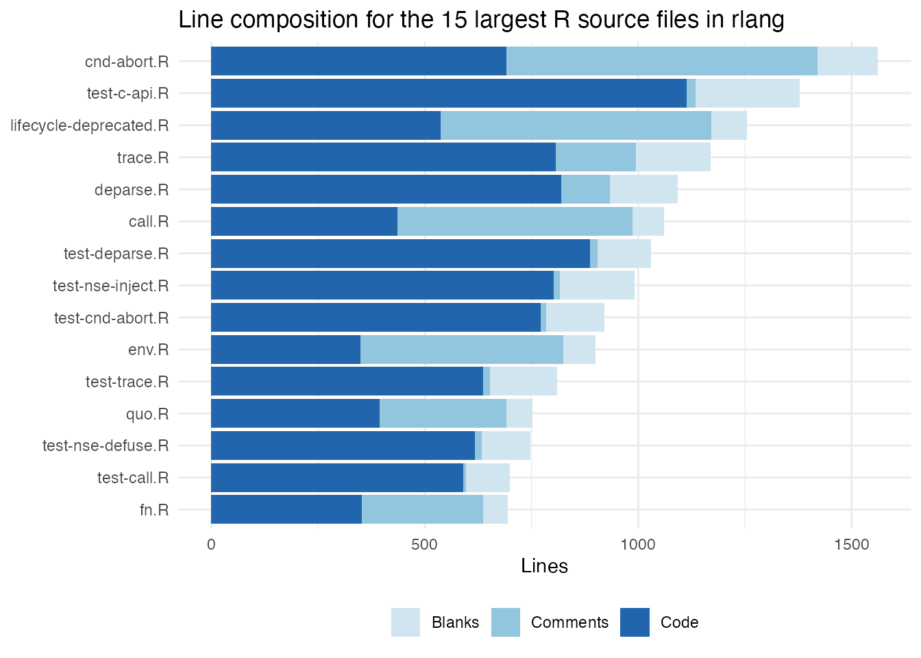
Complexity and ULOC by file
Same files, but now stacking the three per-file numeric metrics that scale with size:
top15cm <- r_files[order(r_files$lines, decreasing = TRUE), ][1:15, ]

tidytop15cm <- tidyr::pivot_longer(
  data      = top15cm,
  cols      = c(complexity, weighted_complexity, uloc),
  names_to  = "c_metric",
  values_to = "value"
)
tidytop15cm$c_metric <- factor(
  tidytop15cm$c_metric,
  levels = c("uloc", "complexity", "weighted_complexity")
)
ggplot2::ggplot(tidytop15cm,
  ggplot2::aes(x = lines, y = reorder(filename, lines), fill = c_metric)) +
  ggplot2::geom_col() +
  ggplot2::scale_fill_manual(
    values = c(weighted_complexity = "#2166ac",
               complexity          = "#92c5de",
               uloc                = "#d1e5f0"),
    labels = c(weighted_complexity = "weighted complexity",
               complexity          = "complexity",
               uloc                = "uloc")
  ) +
  ggplot2::labs(
    title = "ULOC, complexity, and weighted complexity for the 15 largest R files",
    x     = "Lines",
    y     = NULL,
    fill  = NULL
  ) +
  ggplot2::theme_minimal(base_size = 11) +
  ggplot2::theme(legend.position = "bottom")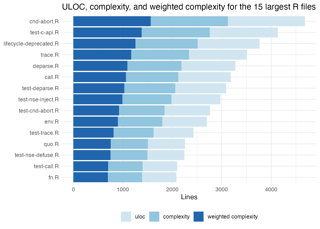
Complexity vs. DRYness as a circle pack
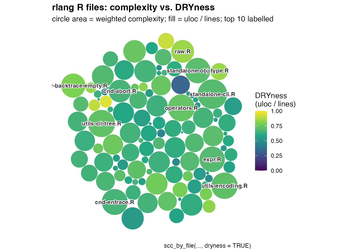
Each circle is one .R source file. The circle area is
the file’s weighted_complexity (complexity per 100 LOC), so
files that pack more branching per line are larger.
The fill color is the file’s dryness
(uloc / lines); darker hues mean more duplication relative
to physical line count, lighter hues mean more unique non-blank
content.
r_files <- scc_by_file(rlang_path, include_ext = "r", dryness = TRUE)Drop files with zero weighted_complexity (nothing to size the circle by).
r_files <- r_files[r_files$weighted_complexity > 0, ]
str(r_files[, c("filename", "weighted_complexity", "dryness")])
#  tibble [109 × 3] (S3: tbl_df/tbl/data.frame)
#   $ filename           : chr [1:109] "standalone-types-check.R" "standalone-lazyeval.R" "operators.R" "cnd-entrace.R" ...
#   $ weighted_complexity: num [1:109] 14.91 16.85 31.03 28.64 7.19 ...
#   $ dryness            : num [1:109] 0.328 0.741 0.731 0.657 0.617 ...
Compute the circle layout with
packcircles::circleProgressiveLayout() (area-proportional
sizing) and turn it into polygon vertices for ggplot2.
Tag every polygon vertex with the filename, weighted complexity, and dryness it belongs to so the static and interactive plots can both render labels:
packing <- packcircles::circleProgressiveLayout(
  r_files$weighted_complexity, sizetype = "area"
)
packing$filename            <- r_files$filename
packing$weighted_complexity <- r_files$weighted_complexity
packing$dryness             <- r_files$dryness
polygons <- packcircles::circleLayoutVertices(packing, npoints = 60)
# circleLayoutVertices() numbered the vertices by the row position of r_files
# polygons$id is being used as a row index into r_files (like a positional join)
polygons$filename            <- r_files$filename[polygons$id]
polygons$weighted_complexity <- r_files$weighted_complexity[polygons$id]
polygons$dryness             <- r_files$dryness[polygons$id]
Static — top-N labelled
To keep the figure readable, only the top 10 circles by weighted complexity get a text label. Smaller circles still render but stay anonymous; their info is recoverable from the interactive version below.
top_labels <- packing[order(-packing$weighted_complexity), ][seq_len(10), ]

ggplot2::ggplot(polygons,
                ggplot2::aes(x, y, group = id, fill = dryness)) +
  ggplot2::geom_polygon(colour = "white", linewidth = 0.2) +
  shadowtext::geom_shadowtext(
    data    = top_labels,
    mapping = ggplot2::aes(x = x, y = y, label = filename),
    inherit.aes = FALSE,
    size      = 3,
    colour    = "#2B2B2B",     # Eames Charcoal (theme `secondary`)
    bg.colour = "white",       # halo so dark text stays legible on dark fills
    bg.r      = 0.15,
    fontface  = "bold"
  ) +
  ggplot2::scale_fill_viridis_c(
    name    = "DRYness\n(uloc / lines)",
    option  = "viridis",
    limits  = c(0, 1)
  ) +
  ggplot2::coord_equal() +
  ggplot2::labs(
    title    = "rlang R files: complexity vs. DRYness",
    subtitle = "circle area = weighted complexity; fill = uloc / lines; top 10 labelled",
    caption  = "scc_by_file(..., dryness = TRUE)"
  ) +
  ggplot2::theme_void(base_size = 11) +
  ggplot2::theme(
    plot.title      = ggplot2::element_text(face = "bold"),
    legend.position = "right"
  )
Interactive — hover every circle
Same layout, but rendered via ggiraph so
each circle is its own SVG element with a tooltip. Hover any circle to
read the file’s name, weighted complexity, and DRYness — including the
small ones that the static plot doesn’t label.
gg_interactive <- ggplot2::ggplot(polygons,
                                  ggplot2::aes(x, y, group = id, fill = dryness)) +
  ggiraph::geom_polygon_interactive(
    mapping = ggplot2::aes(
      tooltip = sprintf(
        "%s\nweighted_complexity: %.2f\ndryness: %.3f",
        filename, weighted_complexity, dryness
      ),
      data_id = id
    ),
    colour    = "white",
    linewidth = 0.2
  ) +
  ggplot2::scale_fill_viridis_c(
    name    = "DRYness\n(uloc / lines)",
    option  = "viridis",
    limits  = c(0, 1)
  ) +
  ggplot2::coord_equal() +
  ggplot2::labs(
    title    = "rlang R files (interactive)",
    subtitle = "hover any circle for filename, weighted complexity, and DRYness"
  ) +
  ggplot2::theme_void(base_size = 11) +
  ggplot2::theme(
    plot.title      = ggplot2::element_text(face = "bold"),
    legend.position = "right"
  )

ggiraph::girafe(
  ggobj         = gg_interactive,
  width_svg     = 7,
  height_svg    = 5,
  options       = list(
    ggiraph::opts_hover(css  = "stroke:#1B2A41; stroke-width:1.5px;"),
    ggiraph::opts_tooltip(opacity = 0.95)
  )
)
The largest circles are the highest-density branching files; comparing their hue tells you whether that complexity is concentrated in repetitive code (low DRYness, dark) or in mostly unique code (high DRYness, bright).