install.packages('remotes')
remotes::install_github("mjfrigaard/glockr")Last week I built glockr, an R package that wraps scc, a “very fast accurate code counter with complexity calculations.” Code metrics are a fascination of mine, and now that code is increasingly written by both machines and humans, I wanted a set of tools I could use for comparison.
Background
Adam Tornhill wrote two books on code metrics: Software Design X-Rays and Your Code as a Crime Scene, 2ed. Both are excellent reads, and were the first exposure I had to any measurements around code complexity.1 The approach to metrics and data visualizations Tornhill outlines has definitely improved the way I think about writing (and maintaining code). He covers topics like essential and accidental complexity, and how often code is changed (i.e., measured via version control) is usually as important as any metrics.
The R ecosystem has some great packages for assessing code quality, too:2
What does glockr do?
glockr wraps the scc command-line tool in an R package (much like cloc). scc is written in pure Go, so it’s much faster than the alternatives.4
Install glockr from GitHub:
We’ll also install gt and dplyr for data manipulation and pretty tables.
install.packages(c('gt', 'dplyr'))library(glockr)
library(gt)
library(dplyr)glockr computes many of the same values of the cloc package, but also includes the weighted complexity, unique lines of code (uloc), and Constructive Cost Model (cocomo) estimates.
Verify that scc is installed with:
scc_version()
## [1] "scc version 3.7.0"The primary function for glockr is scc(). We’ll use the popular rlang package as an example:5
pkg_path <- file.path("rlang/")rlang_scc <- scc(pkg_path)
dplyr::glimpse(rlang_scc)
## Rows: 11
## Columns: 10
## $ language <chr> "R", "Markdown", "C"…
## $ files <int> 163, 53, 70, 72, 9, …
## $ lines <int> 44571, 16935, 14014,…
## $ code <int> 28038, 13866, 10960,…
## $ comments <int> 11152, 0, 872, 1777,…
## $ blanks <int> 5381, 3069, 2182, 11…
## $ complexity <int> 2323, 0, 1851, 691, …
## $ weighted_complexity <dbl> 8.285184, 0.000000, …
## $ bytes <int> 1188357, 496932, 376…
## $ uloc <int> 23837, 5358, 6931, 4…The raw counts in the standard output from scc() includes the following columns:
language: Language of the filefiles: Number of files
lines: Total physical line count across all files (code + comments + blanks)
code: Lines of source code (excludes blanks and comments)
comments: Number of total comments
blanks: Number of total blank lines
bytes: total file size in bytes across all files in that language
Complexity & Weighted Complexity
The complexity calculation in scc is an approximation of the standard cyclomatic complexity:6
“The reason it’s an approximation is that it’s calculated almost for free from a CPU point of view (since its a cheap lookup when counting), whereas a real cyclomatic complexity count would need to parse the code. It gives a reasonable guess in practice though even if it fails to identify recursive methods. The goal was never for it to be exact.
In short when
sccis looking through what it has identified as code if it notices what are usually branch conditions it will increment a counter.”
This approximation is an important limitation if your goal is to compare projects written in different languages. However, if your questions on code quality center around 1) “what are the most complex files in this project?” and – by extension – 2) “what code should be refactored?”, these metrics work well.7
Below is the output from scc() for the rlang source files (sorted by complexity).
rlang_scc |>
dplyr::arrange(desc(complexity)) |>
gt::gt() |>
gt::tab_header(
title = "Succinct Code Count (rlang package)",
subtitle = "Sorted by complexity")| Succinct Code Count (rlang package) | |||||||||
| Sorted by complexity | |||||||||
| language | files | lines | code | comments | blanks | complexity | weighted_complexity | bytes | uloc |
|---|---|---|---|---|---|---|---|---|---|
| R | 163 | 44571 | 28038 | 11152 | 5381 | 2323 | 8.285184 | 1188357 | 23837 |
| C | 70 | 14014 | 10960 | 872 | 2182 | 1851 | 16.888686 | 376444 | 6931 |
| C Header | 72 | 8210 | 5315 | 1777 | 1118 | 691 | 13.000941 | 270950 | 4809 |
| Makefile | 1 | 11 | 7 | 0 | 4 | 2 | 28.571429 | 184 | 8 |
| Markdown | 53 | 16935 | 13866 | 0 | 3069 | 0 | 0.000000 | 496932 | 5358 |
| YAML | 9 | 735 | 587 | 35 | 113 | 0 | 0.000000 | 17940 | 449 |
| C++ | 2 | 25 | 21 | 0 | 4 | 0 | 0.000000 | 492 | 17 |
| C++ Header | 1 | 26 | 21 | 0 | 5 | 0 | 0.000000 | 429 | 21 |
| SVG | 10 | 10 | 10 | 0 | 0 | 0 | 0.000000 | 9687 | 10 |
| License | 1 | 2 | 2 | 0 | 0 | 0 | 0.000000 | 43 | 2 |
| TOML | 1 | 2 | 2 | 0 | 0 | 0 | 0.000000 | 34 | 2 |
This tells us – not surprisingly – that .R code files are the most complex files in this project.
A more useful output is the most complex files in the rlang package, which we can do using:
r_files <- scc_by_file(pkg_path, include_ext = "r")
r_files |>
dplyr::arrange(desc(complexity)) |>
dplyr::select(
c(filename, code, complexity)
) |>
head(10) |>
gt::gt() |>
gt::tab_header(
title = "Top 10 most complex .R files",
subtitle = "raw branch-token count",
preheader = "rlang package")| Top 10 most complex .R files | ||
| raw branch-token count | ||
| filename | code | complexity |
|---|---|---|
| cnd-abort.R | 691 | 152 |
| standalone-cli.R | 432 | 135 |
| trace.R | 807 | 134 |
| deparse.R | 819 | 111 |
| standalone-vctrs.R | 505 | 107 |
| call.R | 451 | 92 |
| standalone-obj-type.R | 206 | 64 |
| cnd-entrace.R | 213 | 61 |
| utils.R | 302 | 59 |
| expr.R | 157 | 52 |
If we compare this to the weighted complexity ((complexity / code) * 100), we can see a few of the top files change:
r_files <- scc_by_file(pkg_path, include_ext = "r")
r_files |>
dplyr::arrange(desc(weighted_complexity)) |>
dplyr::select(
c(filename, code, complexity, weighted_complexity)
) |>
head(10) |>
gt::gt() |>
gt::tab_header(
title = "Top 10 most complex (weighted) .R files",
subtitle = "Weighted Complexity",
preheader = "rlang package")| Top 10 most complex (weighted) .R files | |||
| Weighted Complexity | |||
| filename | code | complexity | weighted_complexity |
|---|---|---|---|
| operators.R | 32 | 11 | 34.37500 |
| expr.R | 157 | 52 | 33.12102 |
| standalone-cli.R | 432 | 135 | 31.25000 |
| standalone-obj-type.R | 206 | 64 | 31.06796 |
| utils-cli-tree.R | 113 | 35 | 30.97345 |
| utils-encoding.R | 37 | 11 | 29.72973 |
| cnd-entrace.R | 213 | 61 | 28.63850 |
| error-backtrace-empty.R | 16 | 4 | 25.00000 |
| raw.R | 9 | 2 | 22.22222 |
| cnd-abort.R | 691 | 152 | 21.99711 |
We won’t spend too much time on these measures, because as you’ll see below, scc has quite a few code metrics to choose from.
Unique lines of code (uloc)
The unique lines of code (ULOC) counts unique non-blank lines including comments. The scc author argues – with help8 – that this is better than relying on SLOC (source lines of code):
“Compared to SLOC, not only are blank lines discounted, but so are close-brace lines and other repetitive code such as common includes. On the other hand, ULOC counts comments, which require just as much maintenance as the code around them does, while avoiding inflating the result with license headers which appear in every file, for example.”
For comparison, SLOC (the value in the code column) is just the raw count of non-blank, non-comment lines and includes duplicates. uloc is automatically included with both scc() and scc_by_file().
The best way to see the differences is with the two minimal code files:
# pure code, 5 lines, two duplicate pairs
# save as code.R
x <- 1
y <- 2
x <- 1
y <- 2
z <- 3# same code, plus three unique comments
# save as code_w_comments.R
# step 1
x <- 1
y <- 2
# step 2
x <- 1
y <- 2
# step 3
z <- 3Now we can compare these with scc_by_file() and view the lines, code, comments and uloc columns.
fixtures <- c(
file.path("code.R"),
file.path("code_w_comments.R")
)
scc_by_file(fixtures) |>
dplyr::select(c(filename, lines,
code, comments, uloc)) |>
gt::gt() |>
gt::tab_header(
title = "SLOC vs ULOC",
subtitle = "Both files contain the same 5 code lines",
preheader = "Local ULOC comparison")| SLOC vs ULOC | ||||
| Both files contain the same 5 code lines | ||||
| filename | lines | code | comments | uloc |
|---|---|---|---|---|
| code.R | 5 | 5 | 0 | 3 |
| code_w_comments.R | 9 | 5 | 4 | 7 |
DRYness percentage
The DRYness % can be added with dryness = TRUE. This is computed locally as uloc / lines, which matches scc’s DRYness % formula, applied per record instead of project-wide.
scc_by_file(fixtures, dryness = TRUE) |>
dplyr::select(c(filename, lines,
code, comments, uloc, dryness)) |>
gt::gt() |>
gt::tab_header(
title = "SLOC vs ULOC + DRYness",
subtitle = "Both files contain the same 5 code lines",
preheader = "Local SLOC, ULOC & DRYness comparison")| SLOC vs ULOC + DRYness | |||||
| Both files contain the same 5 code lines | |||||
| filename | lines | code | comments | uloc | dryness |
|---|---|---|---|---|---|
| code.R | 5 | 5 | 0 | 3 | 0.6000000 |
| code_w_comments.R | 9 | 5 | 4 | 7 | 0.7777778 |
DRYness values close to 1 mean a file or language is mostly unique non-blank content and values closer to 0 mean heavy duplication, comments, or blanks.
COCOMO cost estimates
scc includes a COCOMO 81 model that estimates project effort and cost from SLOC. When cocomo = TRUE, the scc() output becomes a list and the COCOMO output is in the cocomo tibble.
rlang_cocomo <- scc(pkg_path, cocomo = TRUE)
## # A tibble: 11 × 10
## language files lines code comments blanks
## <chr> <int> <int> <int> <int> <int>
## 1 R 163 44571 28038 11152 5381
## 2 Markdown 53 16935 13866 0 3069
## 3 C 70 14014 10960 872 2182
## 4 C Header 72 8210 5315 1777 1118
## 5 YAML 9 735 587 35 113
## 6 C++ 2 25 21 0 4
## 7 C++ Header 1 26 21 0 5
## 8 SVG 10 10 10 0 0
## 9 Makefile 1 11 7 0 4
## 10 License 1 2 2 0 0
## 11 TOML 1 2 2 0 0
## # ℹ 4 more variables: complexity <int>,
## # weighted_complexity <dbl>, bytes <int>,
## # uloc <int>
## # A tibble: 3 × 3
## metric project_type value
## <chr> <chr> <chr>
## 1 Estimated Cost to Develop organic $1,948,3…
## 2 Estimated Schedule Effort organic 17.72 mo…
## 3 Estimated People Required organic 9.77The scc() output is in the scc tibble:
names(rlang_cocomo)
## [1] "scc" "cocomo"We can customize the COCOMO model with the following arguments:
avg_wage: annual salary in local currency
cocomo_project_type: “organic”, “semi-detached”, or “embedded”
eaf: effort adjustment factor
overhead: corporate overhead multiplier
currency_symbol: symbol shown in the value column
auto_print_scc: skip auto-printing the language tibble
NOTE: These arguments only work when cocomo = TRUE
embedded <- scc(pkg_path,
cocomo = TRUE,
avg_wage = 120000L,
cocomo_project_type = "embedded",
eaf = 1.1,
overhead = 2.0,
currency_symbol = "$",
auto_print_scc = FALSE)
## # A tibble: 3 × 3
## metric project_type value
## <chr> <chr> <chr>
## 1 Estimated Cost to Develop embedded $10,525,…
## 2 Estimated Schedule Effort embedded 18.57 mo…
## 3 Estimated People Required embedded 28.35embedded$cocomo |>
gt::gt() |>
gt::tab_header(
title = "COCOMO",
subtitle = "embedded project",
preheader = "rlang package")| COCOMO | ||
| embedded project | ||
| metric | project_type | value |
|---|---|---|
| Estimated Cost to Develop | embedded | $10,525,311 |
| Estimated Schedule Effort | embedded | 18.57 months |
| Estimated People Required | embedded | 28.35 |
Why not use COCOMO II ???
scc() only gives us raw structural numbers (lines, code, complexity, bytes, etc.), but COCOMO II needs 22 judgement inputs we can’t derive from source code:
- The current COCOMO project types (
"organic"/"semi-detached"/"embedded") don’t translate to COCOMO II. - COCOMO II uses 5 scale factors to esitmate organizational/process attributes
- COCOMO II also uses 17 effort multipliers for product, platform, personnel, and project context
- Every one of these is a six-level human rating about the team, requirements stability, reuse strategy, tool maturity, schedule pressure, etc.
- The only one that might map would be CPLX (product complexity), but COCOMO II’s CPLX is architectural/algorithmic complexity, not McCabe’s cyclomatic.
Visualizing code complexity
In Your Code as a Crime Scene, Tornhill covers a collection of methods for visualizing code, but my favorite is his use of circle packing for identifying “hotspots.” These are described below:
“Each circle represents a part of the system. The more complex a module, as measured by lines of code, the larger the circle. We then use color to serve as an attention magnet for the most critical property: change.” - Adam Tornhill (Your Code as a Crime Scene, 2ed)
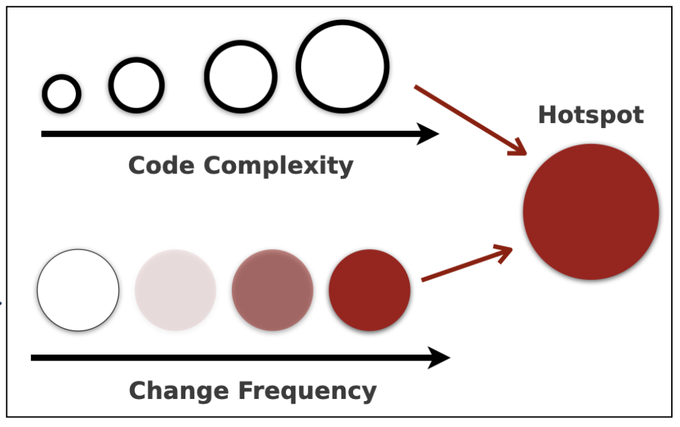
The glockr package doesn’t have data on code changes (yet), but we can build circle packer graphs using weighted complexity and DRYness.
We’ll start by making each circle’s area tied to the file’s weighted_complexity, meaning the files that ‘pack more branching per line’ are larger.
Next, the color fill aesthetic will be the file’s DRYness % (uloc / lines), with darker hues meaning more duplication relative to line counts, and lighter hues meaning more unique, non-blank content.
We’ll start with a fresh dataset using scc_by_file(), setting dryness to TRUE.
r_files <- scc_by_file(pkg_path, include_ext = "r", dryness = TRUE)We can exclude files with zero weighted_complexity because there is nothing to size the circle by:
r_files <- dplyr::filter(r_files, weighted_complexity > 0)
dplyr::glimpse(r_files)
## Rows: 114
## Columns: 14
## $ language <chr> "R", "R", "R", "R", …
## $ filename <chr> "c-lib.R", "aaa-topi…
## $ location <chr> "/Users/mjfrigaard/p…
## $ lines <int> 413, 93, 355, 551, 2…
## $ code <int> 312, 65, 280, 63, 23…
## $ comments <int> 26, 10, 12, 472, 3, …
## $ blanks <int> 75, 18, 63, 16, 40, …
## $ complexity <int> 21, 4, 49, 6, 5, 14,…
## $ weighted_complexity <dbl> 6.7307692, 6.1538462…
## $ bytes <int> 9381, 2708, 10127, 1…
## $ uloc <int> 244, 63, 227, 333, 1…
## $ dryness <dbl> 0.5907990, 0.6774194…
## $ generated <lgl> FALSE, FALSE, FALSE,…
## $ minified <lgl> FALSE, FALSE, FALSE,…The packcircles::circleProgressiveLayout() can be used to compute the area-proportional circle size:
library(packcircles)packing <- packcircles::circleProgressiveLayout(
r_files$weighted_complexity, sizetype = "area"
)This creates a dataset with x, y, and radius columns (with the same number of observations as our previous r_files dataset).
dplyr::glimpse(packing)
## Rows: 114
## Columns: 3
## $ x <dbl> -1.46371800, 1.39958211, 0.052866…
## $ y <dbl> 0.0000000, 0.0000000, -3.5102885,…
## $ radius <dbl> 1.4637180, 1.3995821, 2.3601744, …The number of rows in packing is important, because it allows us to bind the filename, weighted_complexity, and dryness columns back to the packing data:
packing <- dplyr::bind_cols(
packing, # circle size data
dplyr::select(r_files, # original columns
filename, weighted_complexity, dryness)
)
dplyr::glimpse(packing)
## Rows: 114
## Columns: 6
## $ x <dbl> -1.46371800, 1.39958…
## $ y <dbl> 0.0000000, 0.0000000…
## $ radius <dbl> 1.4637180, 1.3995821…
## $ filename <chr> "c-lib.R", "aaa-topi…
## $ weighted_complexity <dbl> 6.7307692, 6.1538462…
## $ dryness <dbl> 0.5907990, 0.6774194…The circleLayoutVertices() function from packcircles creates “a data frame of circle vertices for plotting”
polygons <- packcircles::circleLayoutVertices(packing, npoints = 60)
dplyr::glimpse(polygons)
## Rows: 6,954
## Columns: 3
## $ x <dbl> 0.00000000, -0.00801840, -0.03198575,…
## $ y <dbl> 0.0000000, 0.1530002, 0.3043241, 0.45…
## $ id <int> 1, 1, 1, 1, 1, 1, 1, 1, 1, 1, 1, 1, 1…Now we’re going to perform a positional join using the id from polygons and a new id we’ll create in r_files using dplyr::row_number() (and limit the columns to only filename, weighted_complexity, and dryness).
polygons <- polygons |>
dplyr::left_join(
r_files |>
dplyr::mutate(id = dplyr::row_number()) |>
dplyr::select(
id,
filename,
weighted_complexity,
dryness),
by = "id"
)
dplyr::glimpse(polygons)
## Rows: 6,954
## Columns: 6
## $ x <dbl> 0.00000000, -0.00801…
## $ y <dbl> 0.0000000, 0.1530002…
## $ id <int> 1, 1, 1, 1, 1, 1, 1,…
## $ filename <chr> "c-lib.R", "c-lib.R"…
## $ weighted_complexity <dbl> 6.730769, 6.730769, …
## $ dryness <dbl> 0.590799, 0.590799, …- The
x,y, andgroupaesthetics draw the circles, andfillis thedrynesspercentage value. - The
geom_polygon()is used to connect start and end points (andfillthe area inside)
scale_fill_viridis_c()is used for ‘filling’ continuous data, andcoord_equal()ensures ensures equal unit length on the x-axis and y-axis.
ggplot2::ggplot(polygons,
ggplot2::aes(
x = x,
y = y,
group = id,
fill = dryness)) +
ggplot2::geom_polygon(
colour = "white",
linewidth = 0.2) +
ggplot2::scale_fill_viridis_c(
name = "DRYness\n(uloc / lines)",
option = "viridis",
limits = c(0, 1)
) +
ggplot2::coord_equal() 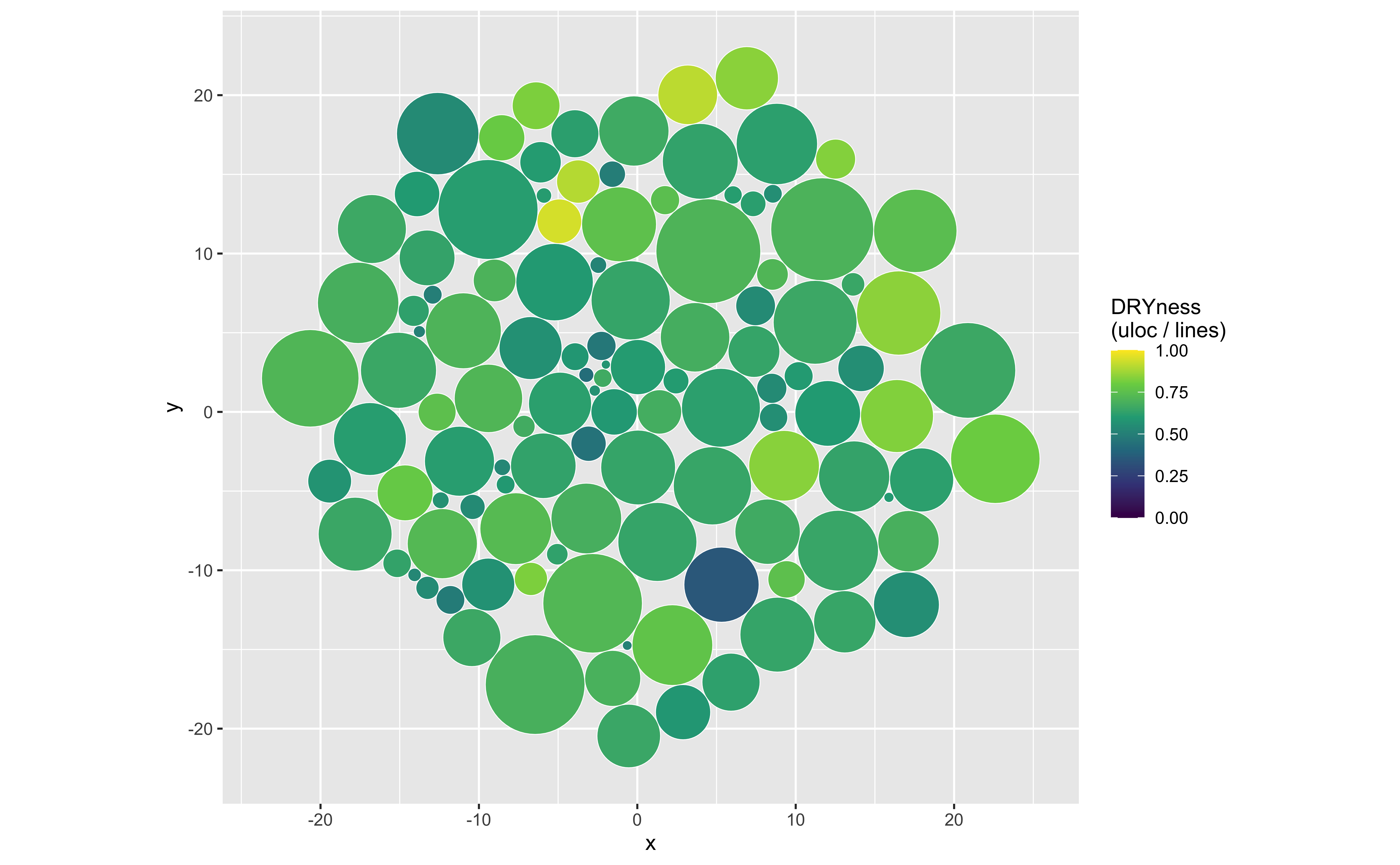
We can’t label every file in the circle packer graph, but we can make sure the files with the highest levels of complexity have text labels. We’ll create a top_labels dataset for the top 10 weighted_complexity values.
top_labels <- packing |>
dplyr::slice_max(weighted_complexity, n = 10)Given the color palette we’re using, we will make sure our labels have a dark outline (behind white text) with the shadowtext package.
remotes::install_github("GuangchuangYu/shadowtext")Now we can add the labels and theme_void():
# for the labels
library(shadowtext)
ggplot2::ggplot(polygons,
ggplot2::aes(
x = x,
y = y,
group = id,
fill = dryness)) +
ggplot2::geom_polygon(
colour = "white",
linewidth = 0.2) +
# add text labels
shadowtext::geom_shadowtext(
data = top_labels,
mapping = ggplot2::aes(
x = x,
y = y,
label = filename),
inherit.aes = FALSE,
size = 3,
colour = "#2B2B2B", # dark text
bg.colour = "white", # white halo so dark text stays legible
bg.r = 0.15,
fontface = "bold"
) +
ggplot2::scale_fill_viridis_c(
name = "DRYness\n(uloc / lines)",
option = "viridis",
limits = c(0, 1)
) +
ggplot2::coord_equal() +
ggplot2::theme_void(base_size = 11)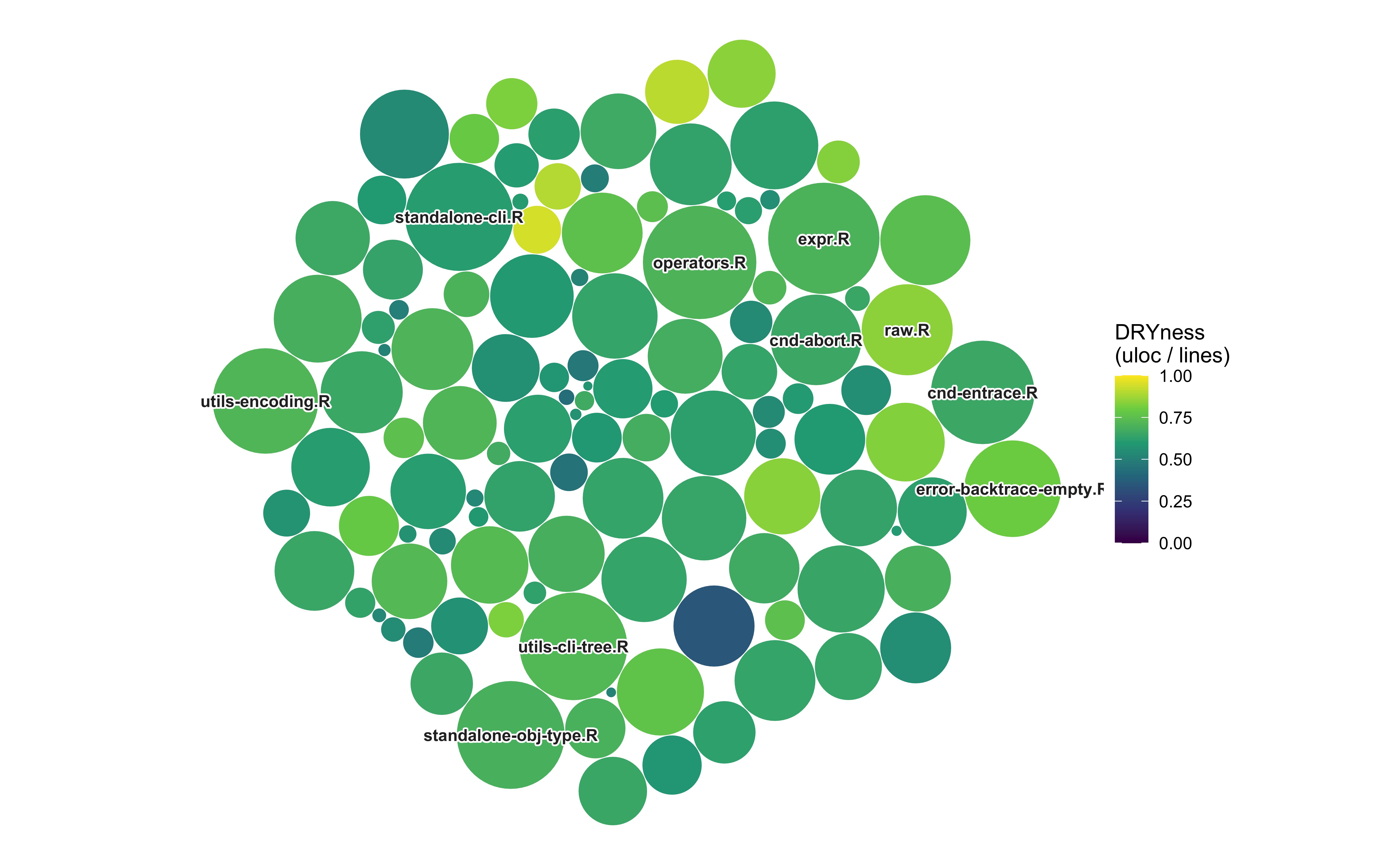
This looks better. I’ll add some finishing touches with lab() and theme():
# for the labels
library(shadowtext)
ggplot2::ggplot(polygons,
ggplot2::aes(
x = x,
y = y,
group = id,
fill = dryness)) +
ggplot2::geom_polygon(
colour = "white",
linewidth = 0.2) +
# add text labels
shadowtext::geom_shadowtext(
data = top_labels,
mapping = ggplot2::aes(x = x, y = y, label = filename),
inherit.aes = FALSE,
size = 3,
colour = "#2B2B2B", # dark text
bg.colour = "white", # white halo so dark text stays legible
bg.r = 0.15,
fontface = "bold"
) +
ggplot2::scale_fill_viridis_c(
name = "DRYness\n(uloc / lines)",
option = "viridis",
limits = c(0, 1)
) +
ggplot2::coord_equal() +
ggplot2::labs(
title = "rlang R files: complexity vs. DRYness",
subtitle = "circle area = weighted complexity; fill = uloc / lines; top 10 labelled",
x = "",
y = "",
caption = "scc_by_file(..., dryness = TRUE)"
) +
ggplot2::theme_void(base_size = 11) +
ggplot2::theme(
plot.title = ggplot2::element_text(face = "bold"),
legend.position = "right"
)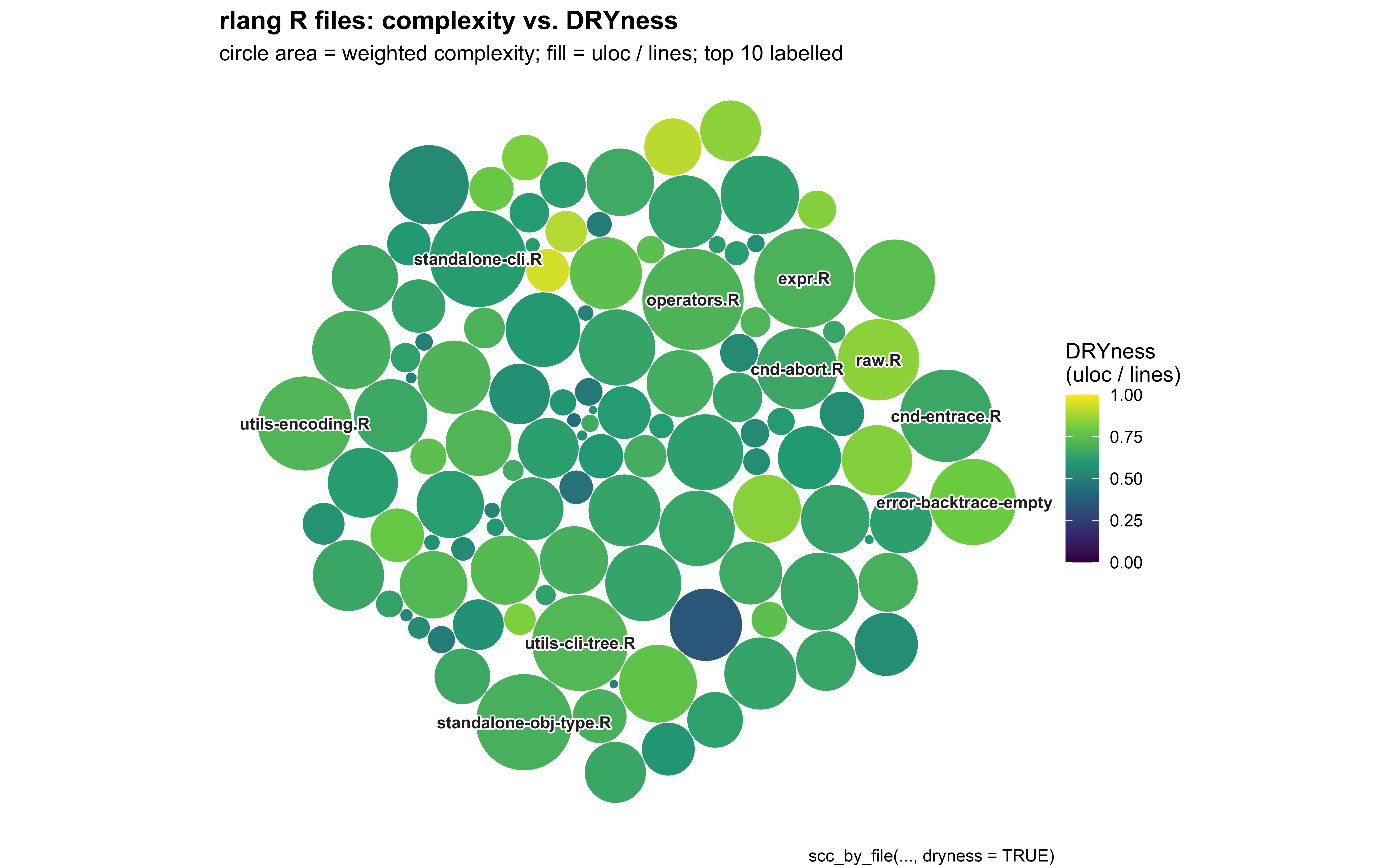
In the Visualization vignette I cover how to convert this into an interactive graph. In future versions, I’ll add the change (Git) data for more interesting hotspot visualizations.
Footnotes
Codacy has a great overview of code metrics in this blog post..↩︎
Other packages worth noting are
sloopandlobstr– these don’t calculate metrics, but have been developed to improve users understanding of R and object oriented programming and are covered in Advanced R, 2nd ed..↩︎This is a downloaded a local version of the source files as of 2026-05-26.↩︎
How
scccounts lines of code is outlined in the ‘Features’ section of theREADME.md↩︎Read the full description of Complexity Estimates.↩︎