ggrewindr is a collection of late 90s ggplot2 themes: Game Boy greens, Surge, Tamagotchi, GeoCities, and 43 more. Each theme samples its palette from a freely licensed image of its reference, and every palette is checked for text contrast and color blind separation. The themes started in fmggp2, the support package for ggplot2: field manual.
Installation
Install the development version from GitHub:
# install.packages("pak")
pak::pak("mjfrigaard/ggrewindr")
Themes
Each theme pairs with simulated data that fits its reference.
| Theme | Reference | Example data |
|---|---|---|
theme_surge() |
Surge | Hexagon bins (cans vs. gaming hours) |
theme_geocities() |
GeoCities | 2D histograms (page load times) |
theme_bopit() |
Bop It | Density contours (reaction times) |
theme_cuseeme() |
CU-SeeMe | Parallel sets (video calls by connection and outcome) |
theme_powerrangers() |
Power Rangers | Grouped bubble charts (putties defeated) |
theme_seinfeld() |
Seinfeld | Bubble charts (Seinfeld episodes) |
theme_consolewars() |
Console wars | Grouped scatter plots (Sega vs. Nintendo) |
theme_doom() |
Doom | Scatter plots (frame rate by CPU speed) |
theme_gushers() |
Fruit Gushers | Instance charts (lunch table trades by year) |
theme_y2k() |
Y2K | Alluvial charts (Y2K prep surveys) |
theme_hypercolor() |
Hypercolor | Stream plots (90s fad sales) |
theme_savedbythebell() |
Saved by the Bell | Slope graphs (Bayside quiz averages) |
theme_visor() |
Handspring Visor | Bump charts (PDA sales rank by year) |
theme_snick() |
SNICK | Grouped line graphs (nightly Nickelodeon ratings) |
theme_batman() |
Batman (1989) | Line graphs (weekly box office) |
theme_rzone() |
Tiger R-Zone | Raincloud plots (seconds to clear the first level) |
theme_aim() |
AOL Instant Messenger | Grouped violin plots (buddy list sizes) |
theme_oregontrail() |
The Oregon Trail | Grouped box plots (days to reach Oregon) |
theme_squeezit() |
Squeezit | Ridgeline plots (seconds to finish a bottle) |
theme_pager() |
Two-way pagers | Overlapping and stacked densities (message lengths by pager) |
theme_tetris() |
Tetris | Beeswarm plots (lines cleared by player) |
theme_goosebumps() |
Goosebumps books | Overlapping dot plots (books read by grade) |
theme_supersoaker() |
Super Soaker | Overlapping frequency polygons (range by model) |
theme_tamagotchi() |
Tamagotchi | Overlapping histograms (virtual pet lifespans) |
theme_j2me() |
J2ME phone games | Treemaps (game downloads by carrier and genre) |
theme_koosh() |
Koosh ball | Pie charts (Koosh ball styles) |
theme_titanic() |
Titanic (1997) | Mosaic plots (moviegoers and viewings) |
theme_netscape() |
Netscape Navigator | Stacked filled densities (modem speeds) |
theme_orbitz() |
Orbitz | Diverging bar graphs (Orbitz vs. Surge survey) |
theme_walkman() |
Sony Walkman Sports | Cleveland dot plots (battery life by model) |
theme_pogs() |
Pogs milk caps | Waffle charts (a collection of 100 Pogs) |
theme_freshprince() |
The Fresh Prince of Bel-Air | Heatmaps (running gags per season) |
theme_netware() |
Novell NetWare | Overlapping bar graphs (LAN protocols by office) |
theme_happymeal() |
McDonald’s Happy Meal box | Summary bar graphs (Happy Meals sold per promotion) |
theme_jurassic() |
Jurassic Park (1993) | Grouped bar graphs (dinosaur weights per paddock) |
theme_n64() |
Nintendo 64 | Box plots (Mario Kart 64 lap times) |
theme_microdrive() |
IBM Microdrive | Violin plots (photo file sizes) |
theme_wired() |
WIRED magazine | Density plots (story reading times) |
theme_blockbuster() |
Blockbuster Video | Dot plots (weekly rentals) |
theme_gameboy() |
Original Game Boy screen | Bar graphs (Pokémon starters) |
theme_oksoda() |
OK Soda | Histograms (cans sold per store) |
theme_talkboy() |
Talkboy | Frequency polygons (recorded message lengths) |
The two graphs below use theme_oksoda() and theme_talkboy() with simulated data.
library(ggrewindr)
library(ggplot2)
showtext::showtext_auto()
showtext::showtext_opts(dpi = 150) # match the figure dpi set above
set.seed(1014)
ok_soda_sales <- data.frame(cans = round(rnorm(300, mean = 45, sd = 12)))
ggplot(ok_soda_sales, aes(x = cans)) +
  geom_histogram(bins = 30) +
  labs(title = "OK Soda", caption = "Simulated data",
       x = "Cans sold per store") +
  theme_oksoda(base_size = 13)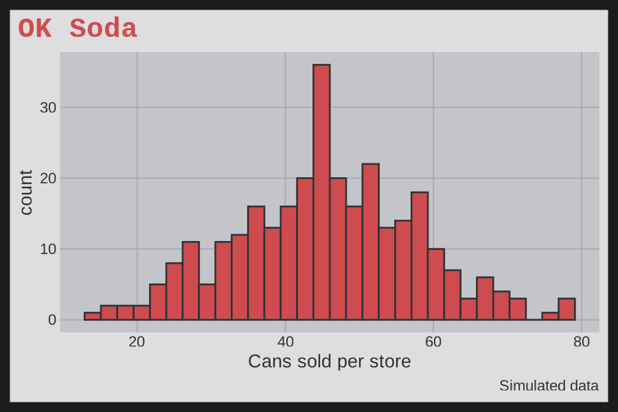
set.seed(1999)
talkboy_clips <- data.frame(seconds = round(rgamma(300, shape = 4, rate = 0.5), 1))
ggplot(talkboy_clips, aes(x = seconds)) +
  geom_freqpoly(bins = 30) +
  labs(title = "Talkboy", caption = "Simulated data",
       x = "Message length (seconds)") +
  theme_talkboy(base_size = 13)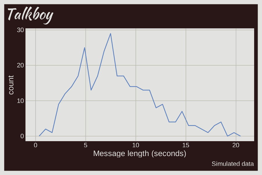
Reference images
Each theme’s palette is sampled from a photo or screenshot of its 90s reference. The themes vignette shows each image with its author and license, and only images licensed for reuse (public domain, CC0, CC BY, or CC BY-SA) are included. A few themes, like theme_goosebumps(), don’t have a freely licensed image yet, so the vignette shows their graphs without one.