Each ggrewindr theme is built around a late 90s toy, snack, TV show, or piece of technology. This vignette shows every theme with simulated data to match its reference.
Themes with a dark background also have a light version. Set mode = "light" to get a light background with darker text and marks. Dark is the default. Each dark theme’s section below shows both versions.
3Com Audrey
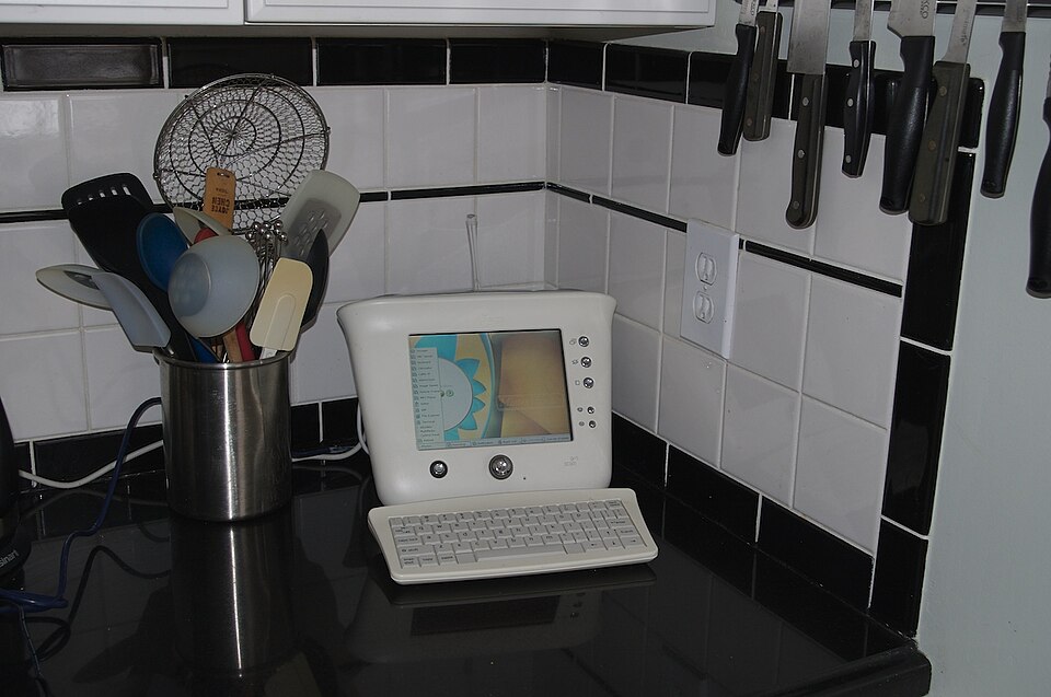
theme_audrey() uses a 3Com Audrey on a kitchen counter: a white plastic background, a black tile frame, teal, navy, tan, brown, and aqua marks, and a teal Varela Round title. Below we simulate what 300 households used their Audrey for.
set.seed(2000)
uses <- data.frame(month = rep(c("Oct", "Nov", "Dec"), each = 300),
  task = sample(c("Email", "Weather", "Recipes", "Calendar", "Browsing"), 900, replace = TRUE))
uses$month <- factor(uses$month, levels = c("Oct", "Nov", "Dec"))
ggplot(uses, aes(x = month, fill = task)) +
  geom_bar(position = "fill") +
  labs(title = "Audrey at home", caption = "Simulated data", x = NULL, y = "Share of households", fill = NULL) +
  theme_audrey(base_size = 13)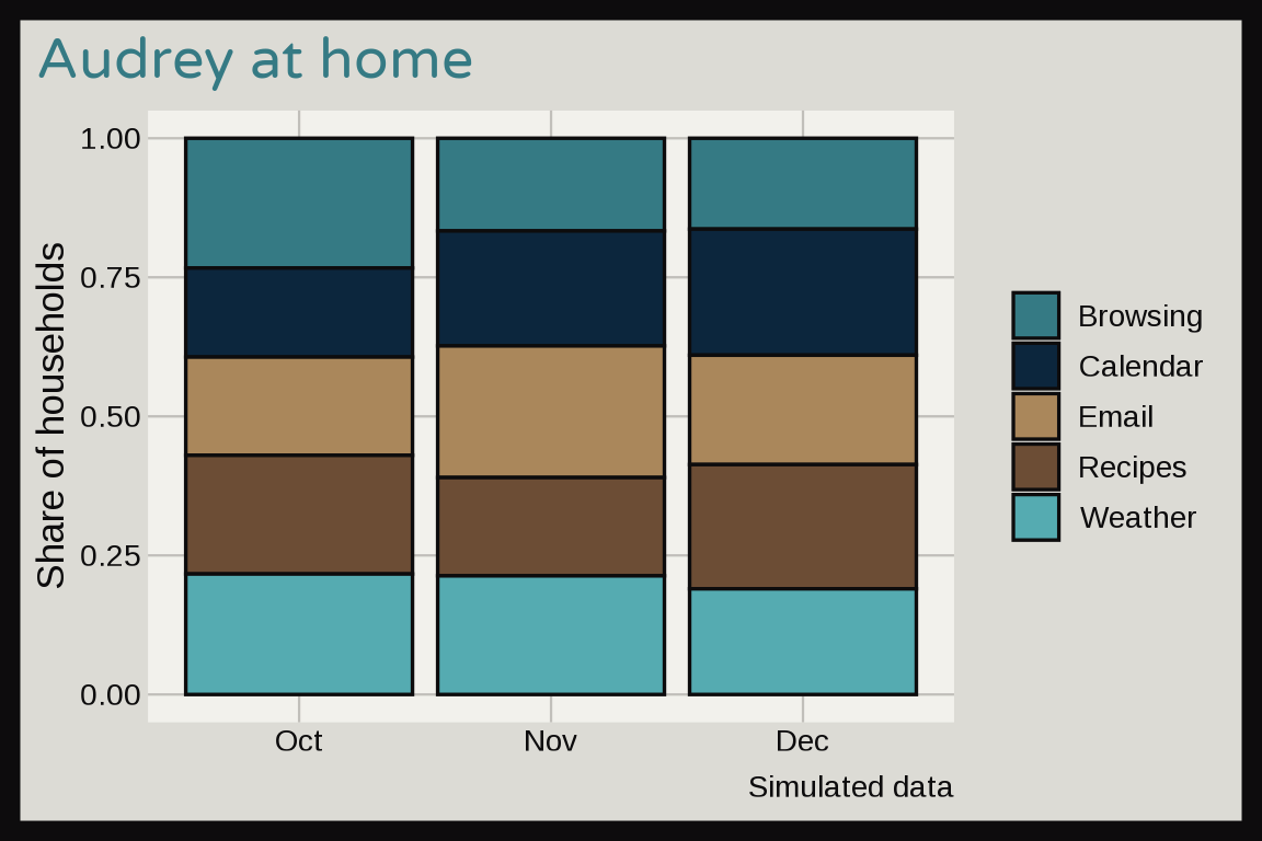
AIM
theme_aim(): the sign on window’s gray, AOL blue, sky blue, and the yellow running man. Below we simulate buddy list sizes with different shapes.

set.seed(1997)
buddies <- data.frame(school = rep(c("Middle school", "College"), each = 150))
buddies$n <- ifelse(buddies$school == "Middle school", rpois(300, 20), ifelse(runif(300) < 0.7, rnorm(300, 60, 10), rnorm(300, 150, 20)))
ggplot(buddies, aes(x = school, y = n, fill = school)) +
  geom_violin(alpha = 2/3, show.legend = FALSE) +
  labs(title = "AIM buddy lists (simulated)", x = NULL, y = "Buddies") +
  theme_aim(base_size = 13)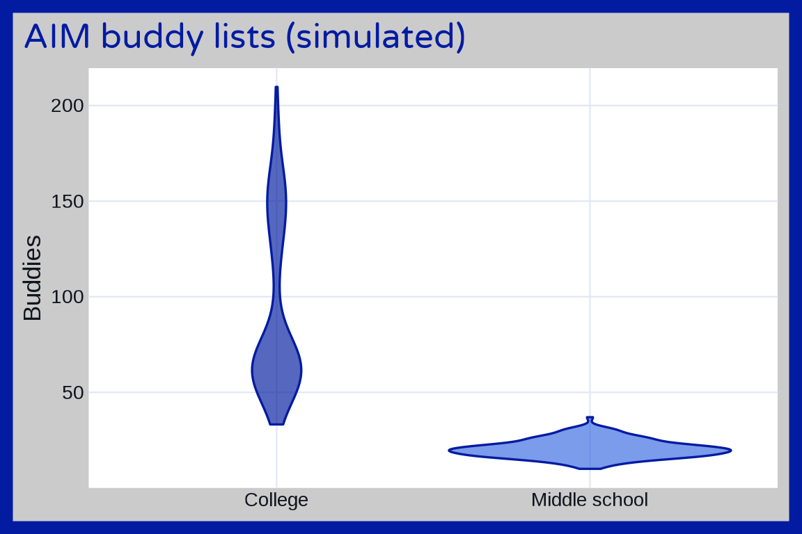
Batman
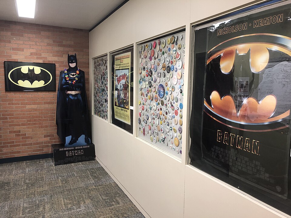
theme_batman() comes in three versions. The default, version = "movie", uses the Batman (1989) palette: black, gold, orange, and steel. Below we simulate bat signal sightings over a week.
set.seed(1989)
signals <- data.frame(night = factor(c("Mon", "Tue", "Wed", "Thu", "Fri", "Sat", "Sun"), levels = c("Mon", "Tue", "Wed", "Thu", "Fri", "Sat", "Sun")), sightings = rpois(7, 12))
ggplot(signals, aes(x = night, y = sightings)) +
  geom_col() +
  labs(title = "Bat signal sightings (simulated)", x = NULL, y = "Sightings") +
  theme_batman(base_size = 13)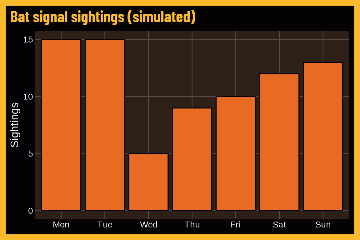
With mode = "light":
last_plot() + theme_batman(base_size = 13, mode = "light")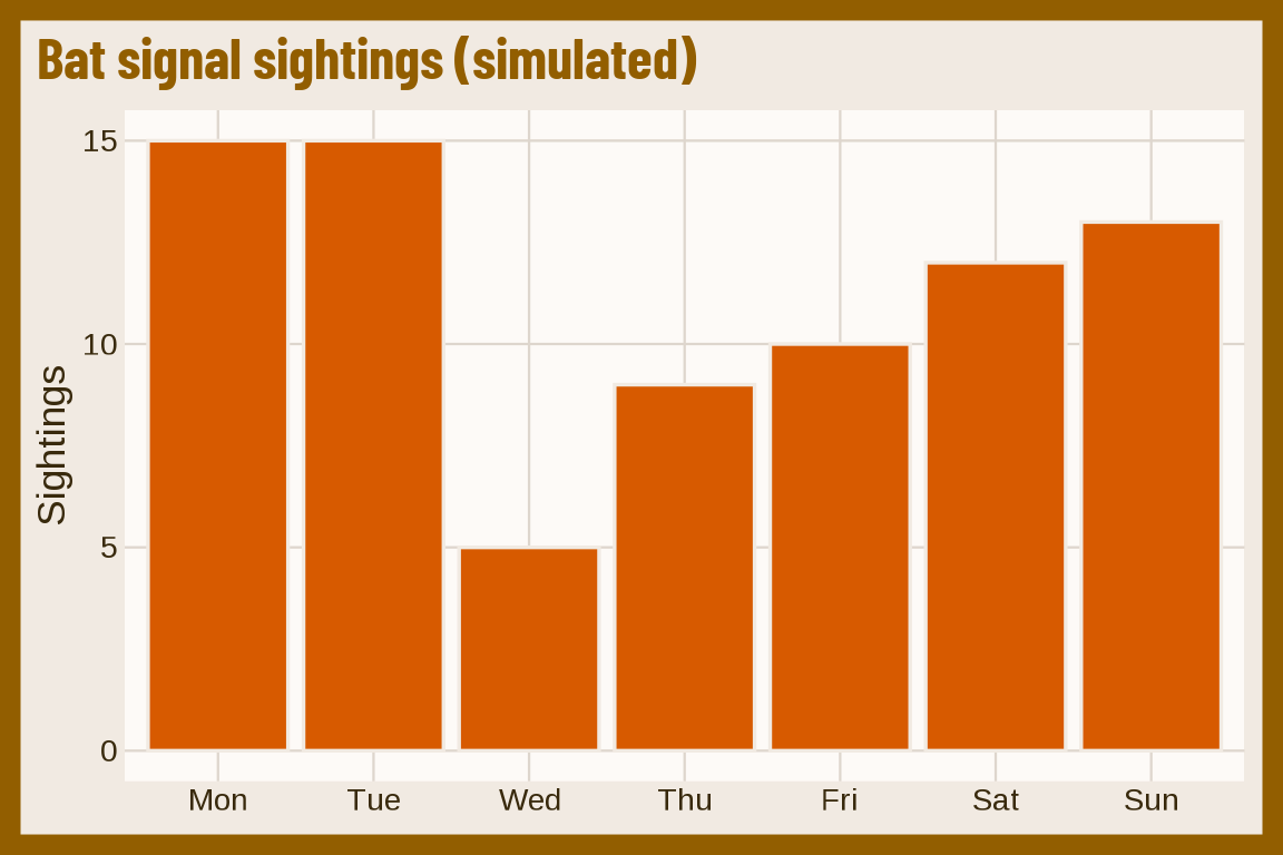
version = "classic" uses the 1966 TV series palette: gray, blue, yellow, black, and cream.

ggplot(signals, aes(x = night, y = sightings)) +
  geom_col() +
  labs(title = "Bat signal sightings (simulated)", x = NULL, y = "Sightings") +
  theme_batman(base_size = 13, version = "classic")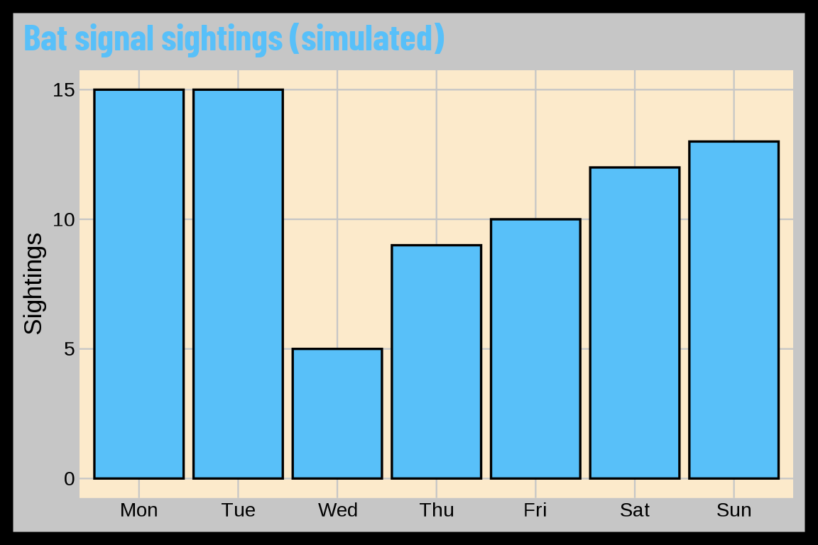
version = "darknight" uses The Dark Knight palette: yellow, olive, charcoal, navy, and slate.

ggplot(signals, aes(x = night, y = sightings)) +
  geom_col() +
  labs(title = "Bat signal sightings (simulated)", x = NULL, y = "Sightings") +
  theme_batman(base_size = 13, version = "darknight")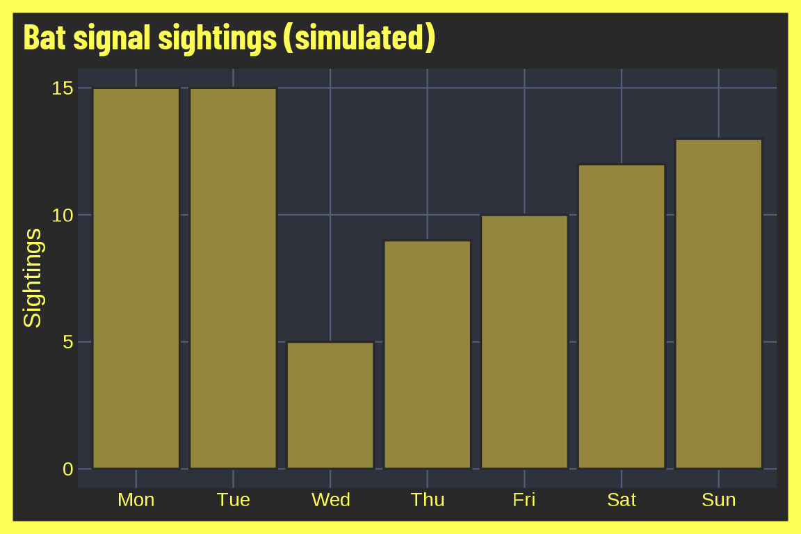
With mode = "light":
last_plot() + theme_batman(base_size = 13, version = "darknight", mode = "light")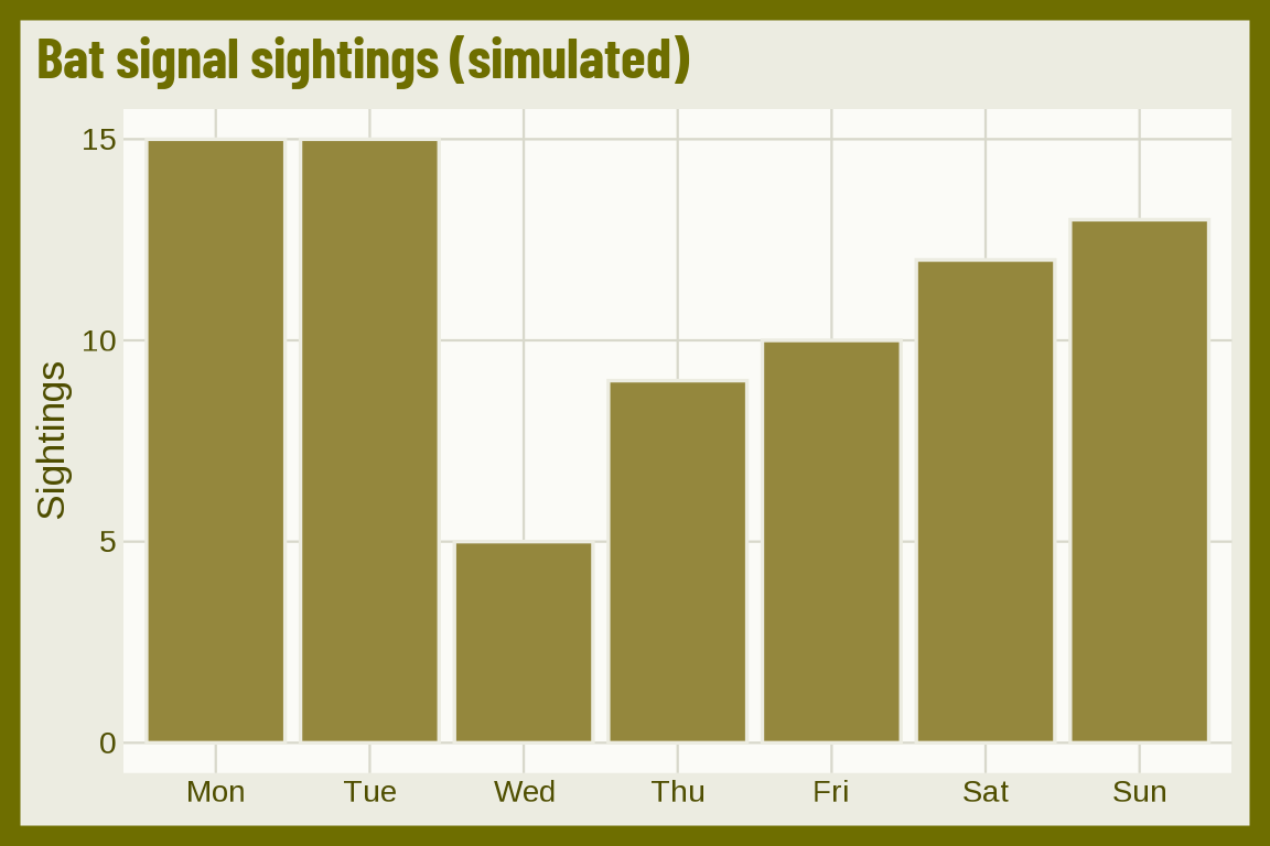
Blockbuster
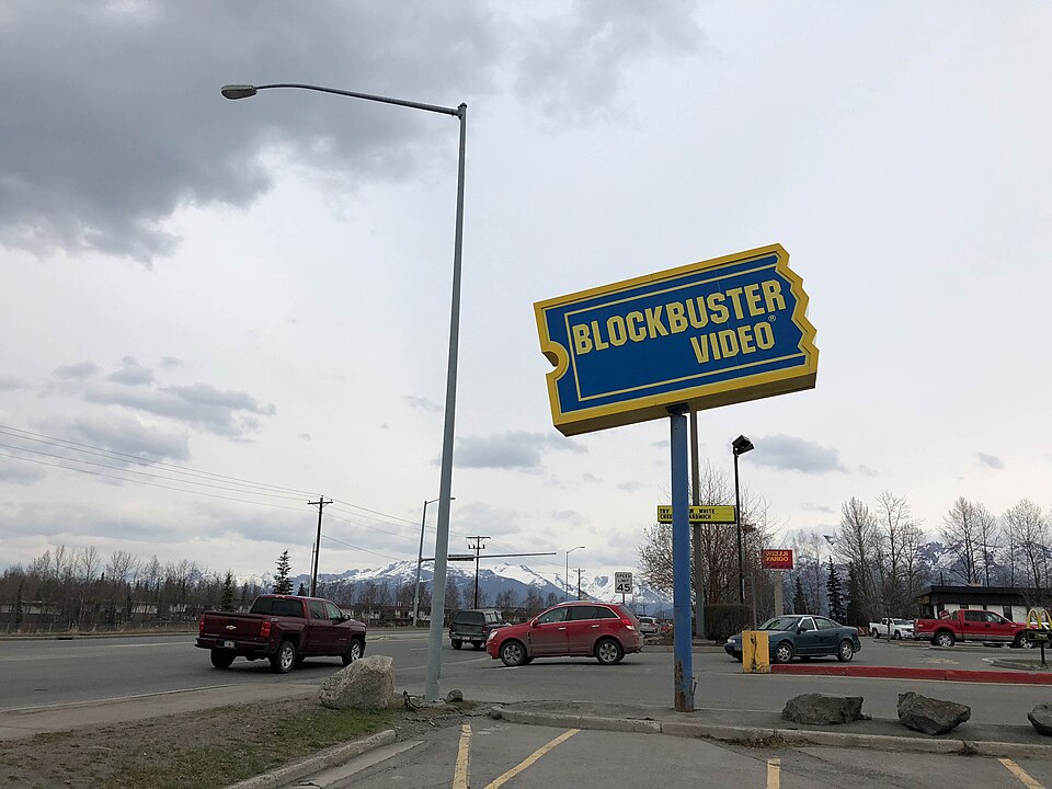
theme_blockbuster() uses Blockbuster Video blue and yellow. Below we simulate weekly rentals for 60 households from a Poisson distribution.
set.seed(1993)
blockbuster_rentals <- data.frame(rentals = rpois(n = 60, lambda = 3))
ggplot(blockbuster_rentals, aes(x = rentals)) +
  geom_dotplot(binwidth = 1, dotsize = 0.3) +
  labs(title = "Blockbuster Video (simulated)",
       x = "Number of rentals") +
  theme_blockbuster(base_size = 13)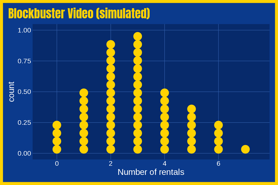
With mode = "light":
last_plot() + theme_blockbuster(base_size = 13, mode = "light")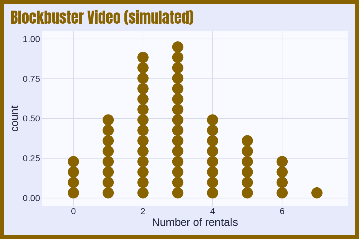
Bop It
theme_bopit(): Bop It yellow on deep purple, with a purple to yellow continuous scale. Below we simulate reaction times to two commands.

set.seed(1996)
players <- data.frame(bop = rnorm(300, 450, 60))
players$twist <- 60 + 0.9 * players$bop + rnorm(300, 0, 40)
ggplot(players, aes(x = bop, y = twist)) +
  geom_point(aes(color = twist), show.legend = FALSE) +
  labs(title = "Bop It reaction times", caption = "Simulated data", x = "Bop it! (ms)", y = "Twist it! (ms)") +
  theme_bopit(base_size = 13)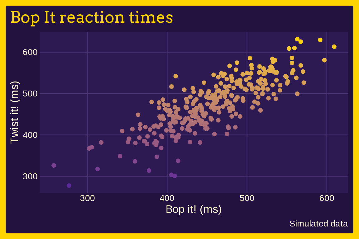
With mode = "light":
last_plot() + theme_bopit(base_size = 13, mode = "light")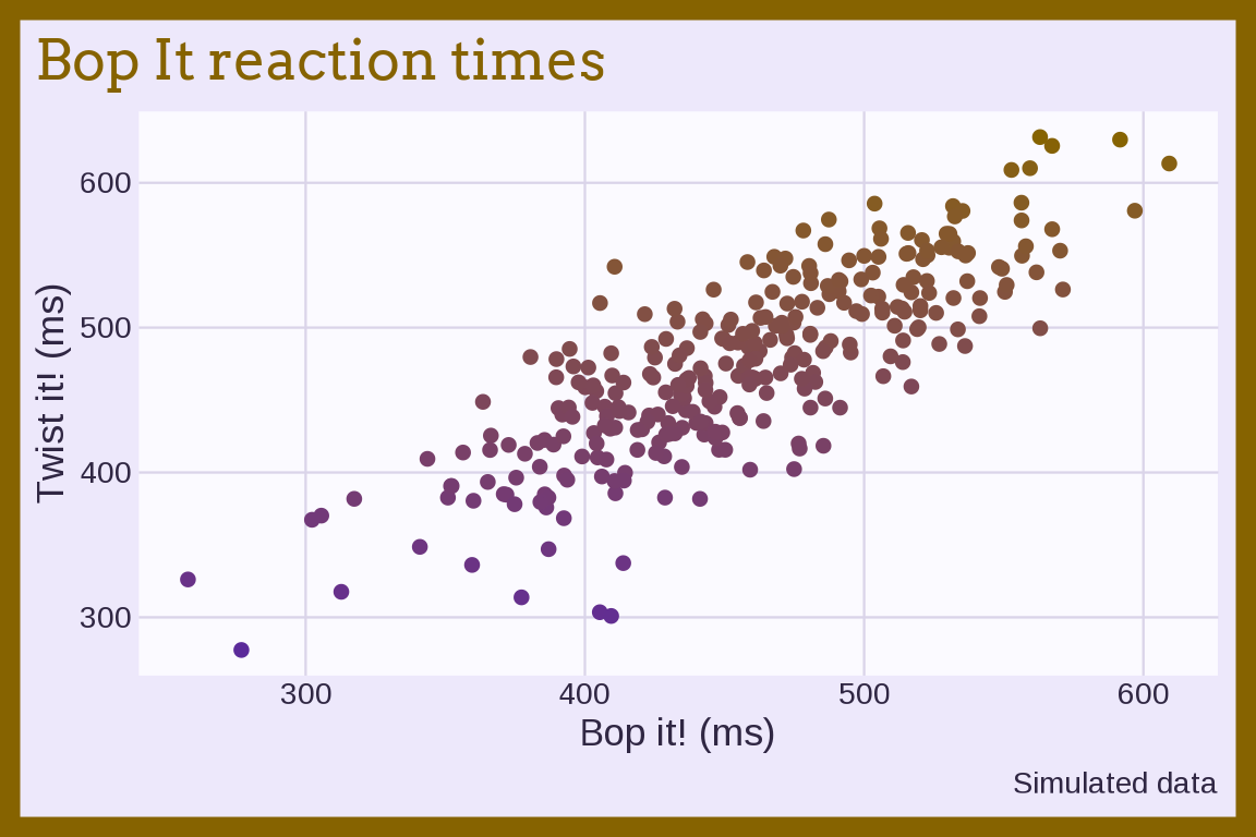
Console wars
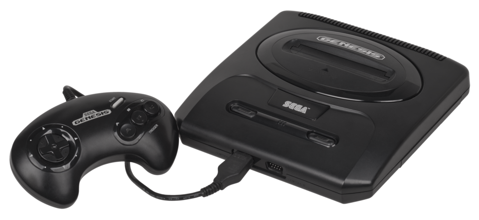
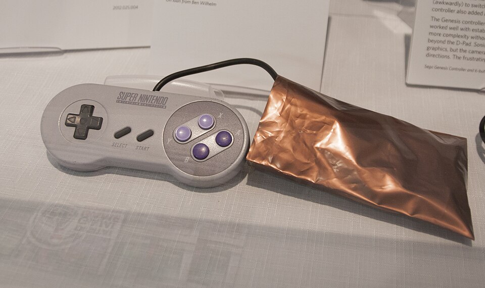
theme_consolewars(): Sega blue vs. Nintendo red on charcoal. Below we simulate games owned and hours played for two consoles.
set.seed(1991)
kids <- data.frame(console = rep(c("Genesis", "SNES"), each = 60), games = rnorm(120, 11, 3))
kids$hours <- 2 + 0.6 * kids$games + ifelse(kids$console == "SNES", 2, 0) + rnorm(120, 0, 2)
ggplot(kids, aes(x = games, y = hours, color = console)) +
  geom_point() +
  labs(title = "The console wars", caption = "Simulated data", x = "Games owned", y = "Hours per week", color = NULL) +
  theme_consolewars(base_size = 13)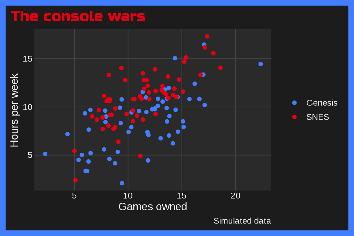
With mode = "light":
last_plot() + theme_consolewars(base_size = 13, mode = "light")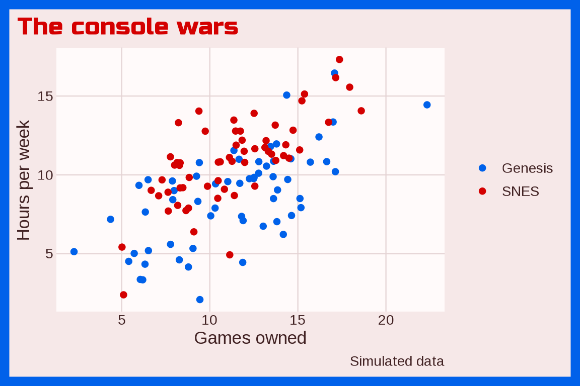
CU-SeeMe
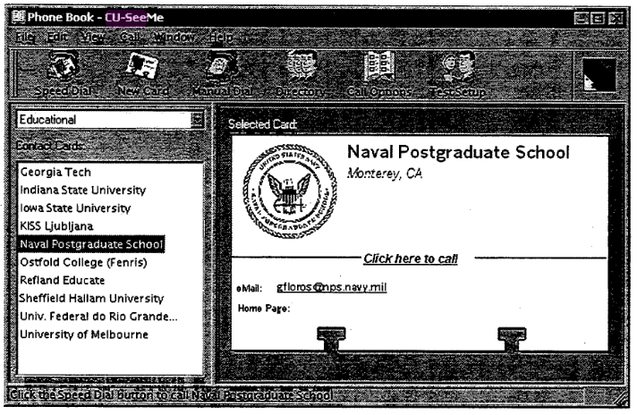
theme_cuseeme() uses the CU-SeeMe phone book window: a dithered gray background, a black frame, a white panel, black, magenta, and gray marks, and a magenta Noto Sans title. Below we simulate video call frame rates over three kinds of connections.
set.seed(1995)
calls <- data.frame(connection = rep(c("28.8k modem", "ISDN", "T1"), each = 60))
calls$fps <- pmax(0.5, rnorm(180, c("28.8k modem" = 2, "ISDN" = 6, "T1" = 14)[calls$connection], 1.5))
ggplot(calls, aes(x = connection, y = fps, color = connection)) +
  geom_jitter(width = 0.2, show.legend = FALSE) +
  labs(title = "CU-SeeMe frame rates", caption = "Simulated data", x = NULL, y = "Frames per second") +
  theme_cuseeme(base_size = 13)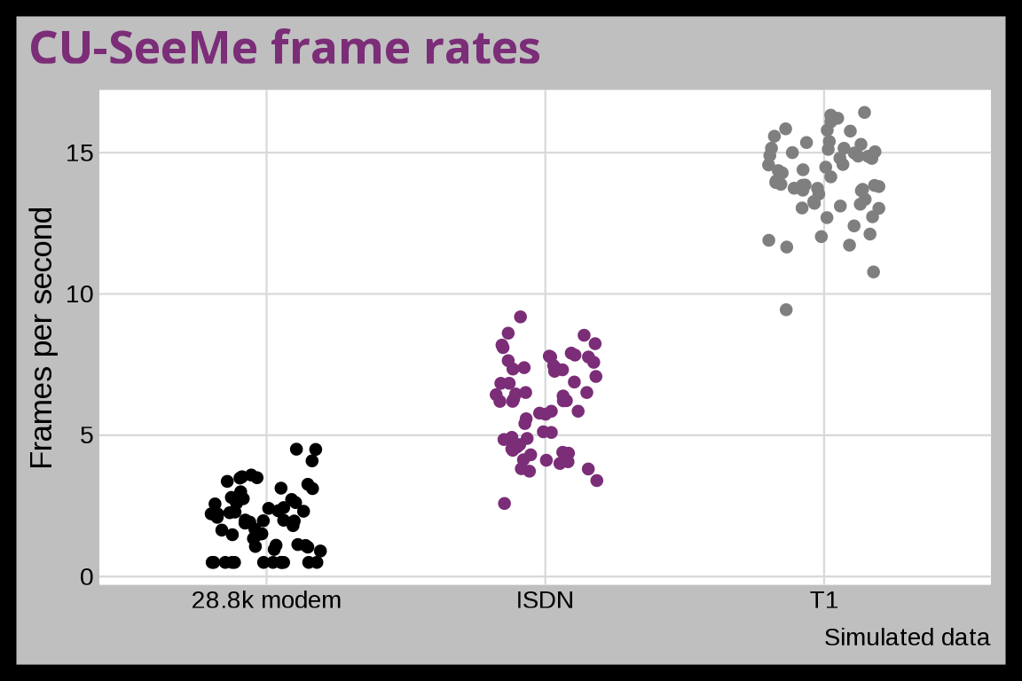
CueCat
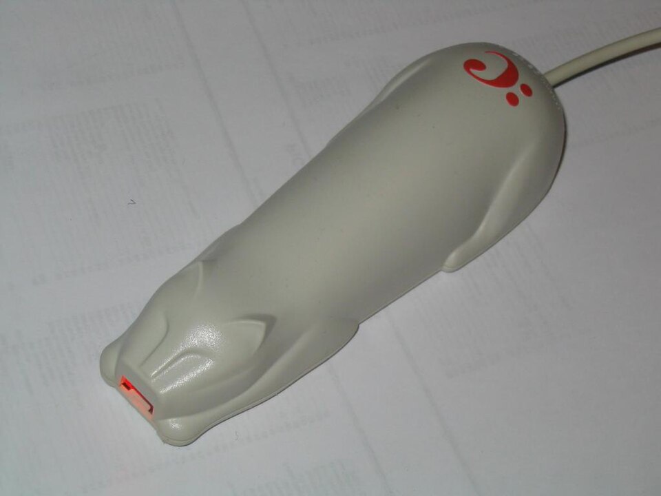
theme_cuecat() uses the :CueCat barcode scanner: a pale paper background, a putty frame, red, ink, LED orange, and putty marks, and a red Permanent Marker title. Below we simulate weekly barcode scans after the free scanners shipped in 2000.
set.seed(2000)
scans <- data.frame(week = 1:52)
scans$scans <- rpois(52, 5000 * exp(-scans$week / 10))
ggplot(scans, aes(x = week, y = scans)) +
  geom_area(alpha = 0.8) +
  labs(title = "CueCat scans", caption = "Simulated data", x = "Week", y = "Barcodes scanned") +
  theme_cuecat(base_size = 13)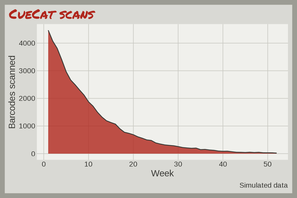
Doom
theme_doom(): hellfire red and orange on scorched brown. Below we simulate Doom frame rates by processor speed.

set.seed(1993)
pcs <- data.frame(mhz = runif(100, 25, 100))
pcs$fps <- pmin(35, 0.45 * pcs$mhz + rnorm(100, 0, 3))
ggplot(pcs, aes(x = mhz, y = fps)) +
  geom_point() +
  labs(title = "Doom frame rates", caption = "Simulated data", x = "CPU (MHz)", y = "Frames per second") +
  theme_doom(base_size = 13)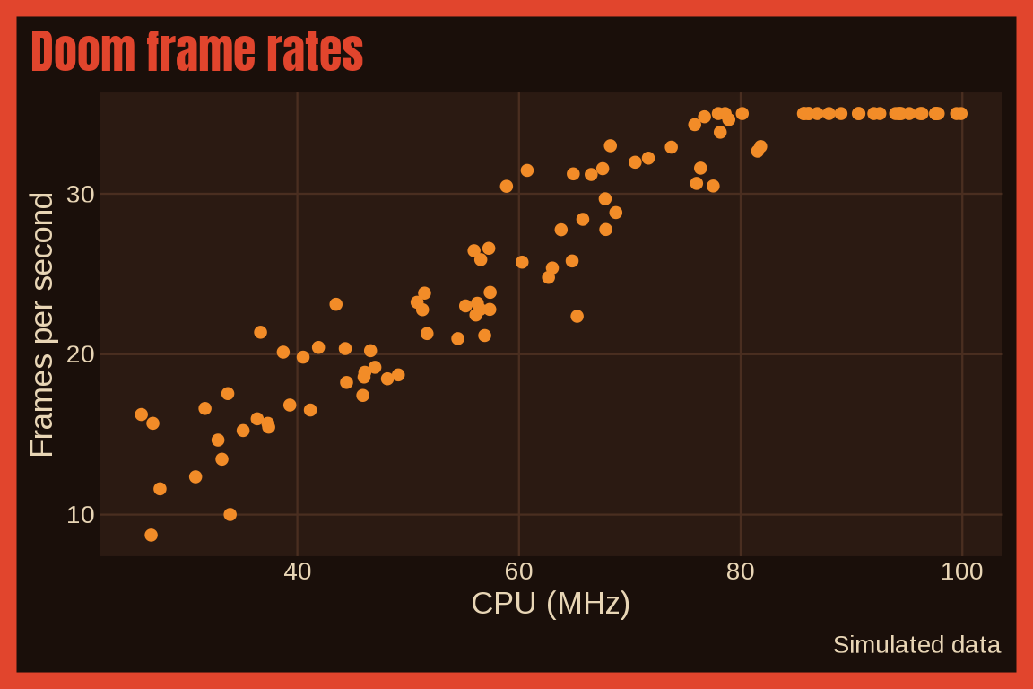
With mode = "light":
last_plot() + theme_doom(base_size = 13, mode = "light")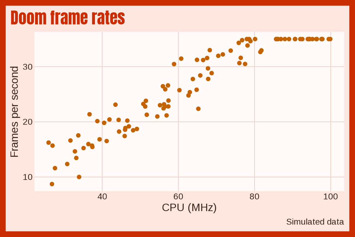
Fresh Prince
theme_freshprince() uses The Fresh Prince of Bel-Air logo: graffiti greens on a pink glow, with a continuous fill that runs from teal to lime. Below we simulate how often the Carlton dance shows up each season.
set.seed(1990)
fp <- expand.grid(season = 1:6, gag = c("Will flirts", "Carlton dance"))
fp$occurrences <- rbinom(12, 24, ifelse(fp$gag == "Will flirts", 0.9, plogis(-2.2 + 0.5 * (fp$season - 3.5))))
ggplot(fp, aes(x = season, y = gag, fill = occurrences)) +
  geom_tile() +
  labs(title = "Fresh Prince (simulated)", x = "Season", y = NULL, fill = "Episodes") +
  theme_freshprince(base_size = 13)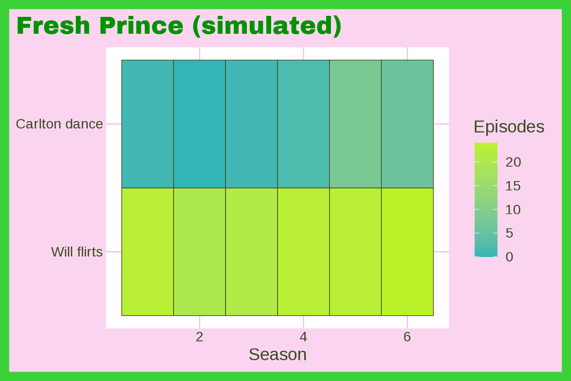
Fruit Gushers
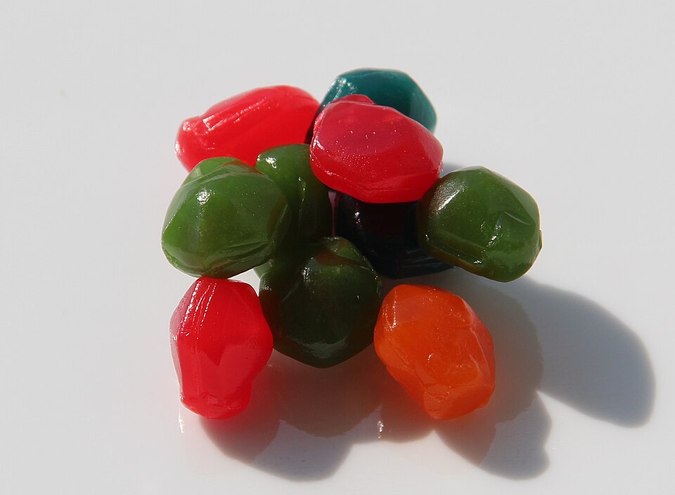
theme_gushers() uses a pile of Fruit Gushers on a white plate: a red frame and title, red, green, teal, orange, and pink marks, and a Patrick Hand title. Below we simulate fruit snack trades at one lunch table before and after Gushers arrived in 1991.
set.seed(1993)
trades <- expand.grid(year = 1985:2000, flavor = c("Strawberry", "Lime", "Blue raspberry"))
trades$n <- rpois(nrow(trades), ifelse(trades$year < 1991, 0.5, 3))
ggplot(subset(trades, n > 0), aes(x = year, y = flavor, color = flavor, alpha = n)) +
  geom_point(shape = 124, size = 6, show.legend = FALSE) +
  labs(title = "Fruit Gushers", caption = "Simulated data", x = NULL, y = NULL) +
  theme_gushers(base_size = 13)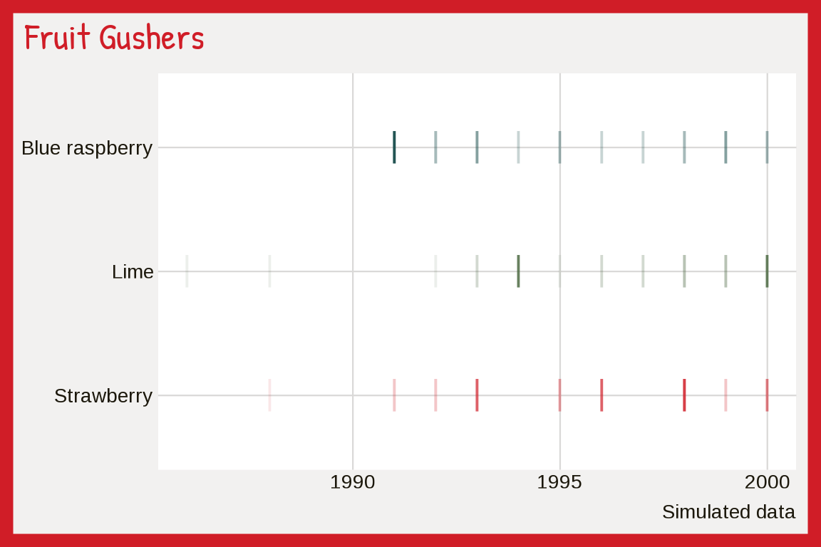
Game Boy
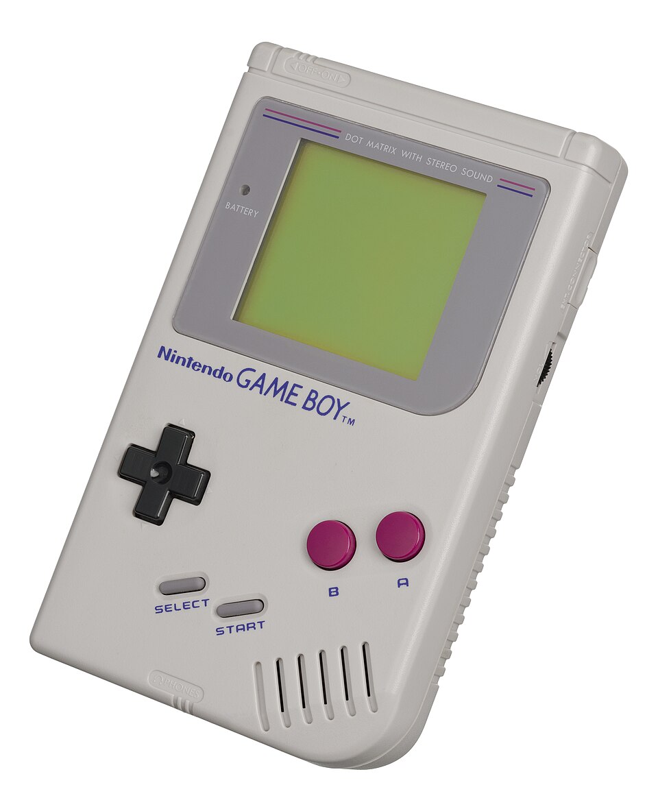
theme_gameboy() uses the four shades of green from the original Game Boy screen and the pixel font Press Start 2P, which ships with ggrewindr. Below we simulate the starter chosen by 300 Pokémon Red and Blue players.
set.seed(1998)
pokemon_starters <- data.frame(
  starter = sample(c("Bulbasaur", "Charmander", "Squirtle"),
    size = 300, replace = TRUE, prob = c(0.30, 0.42, 0.28))
)
ggplot(pokemon_starters, aes(x = starter, fill = starter)) +
  geom_bar(show.legend = FALSE) +
  labs(title = "Pokemon Red and Blue (simulated)",
       subtitle = "Starter chosen by 300 players",
       x = "Starter", y = "Count") +
  theme_gameboy(base_size = 13)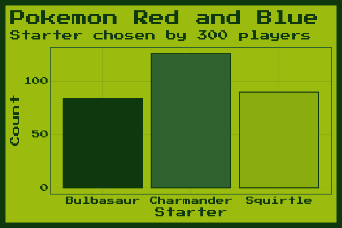
GeoCities
theme_geocities(): lime text and a yellow Comic Neue title on a dark navy panel. Below we simulate GeoCities page loads.

set.seed(1997)
pages <- data.frame(kb = rlnorm(2000, log(60), 0.45))
pages$seconds <- 2 + pages$kb * 8 / 44 + rnorm(2000, 0, 1.5)
ggplot(pages, aes(x = kb, y = seconds)) +
  geom_bin2d(bins = 25) +
  labs(title = "GeoCities page loads", caption = "Simulated data", x = "Page size (KB)", y = "Seconds to load") +
  theme_geocities(base_size = 13)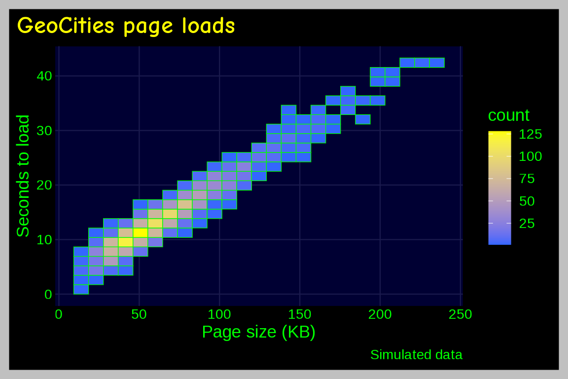
With mode = "light":
last_plot() + theme_geocities(base_size = 13, mode = "light")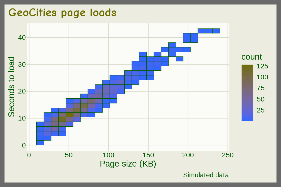
Goosebumps
theme_goosebumps(): the slime green logo and purple covers of the Goosebumps books on black, with a Uncial Antiqua title. Below we simulate Goosebumps books read by two grades.
set.seed(1992)
readers <- data.frame(grade = rep(c("3rd grade", "5th grade"), each = 40))
readers$books <- rpois(80, ifelse(readers$grade == "3rd grade", 3, 9))
ggplot(readers, aes(x = books, fill = grade)) +
  geom_dotplot(method = "histodot", binwidth = 1, stackgroups = TRUE, binpositions = "all") +
  labs(title = "Goosebumps (simulated)", x = "Books read", fill = "Grade") +
  theme_goosebumps(base_size = 13)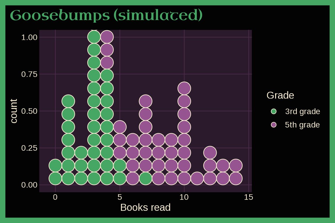
With mode = "light":
last_plot() + theme_goosebumps(base_size = 13, mode = "light")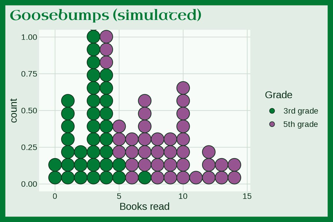
Handspring Visor
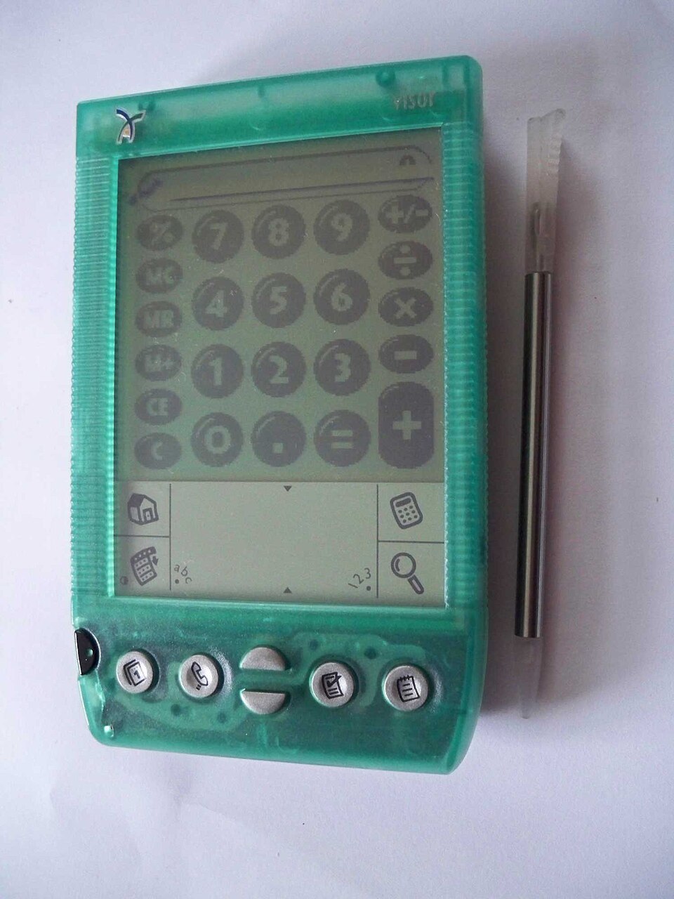
theme_visor() uses a green Handspring Visor Deluxe: a pale lavender background, a translucent green frame, a gray LCD panel, green, gray, mint, and silver marks, and a Fira Sans title. Below we simulate sales of four Springboard modules.
set.seed(2000)
modules <- data.frame(module = sample(c("Games", "MP3 player", "Modem", "Phone"),
  size = 500, replace = TRUE, prob = c(0.35, 0.25, 0.25, 0.15)))
ggplot(modules, aes(y = module, fill = module)) +
  geom_bar(show.legend = FALSE) +
  labs(title = "Springboard modules", caption = "Simulated data", x = "Modules sold", y = NULL) +
  theme_visor(base_size = 13)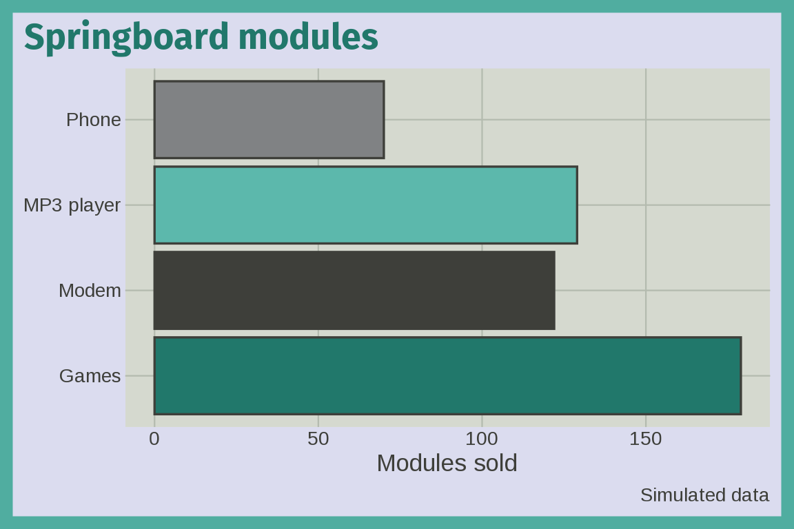
Happy Meals
theme_happymeal() uses the red and yellow of a Happy Meal box. Below we simulate average daily Happy Meal sales for four toy promotions.
set.seed(1997)
happy_meals <- data.frame(promotion = c("Teenie Beanie Babies", "Furby", "Hot Wheels", "Inspector Gadget"),
  avg_sold = sapply(c(420, 310, 220, 180), function(l) mean(rpois(28, l))))
ggplot(happy_meals, aes(x = promotion, y = avg_sold, fill = promotion)) +
  geom_col(show.legend = FALSE) +
  labs(title = "Happy Meals (simulated)", x = "Toy promotion", y = "Average sold per day") +
  theme_happymeal(base_size = 13)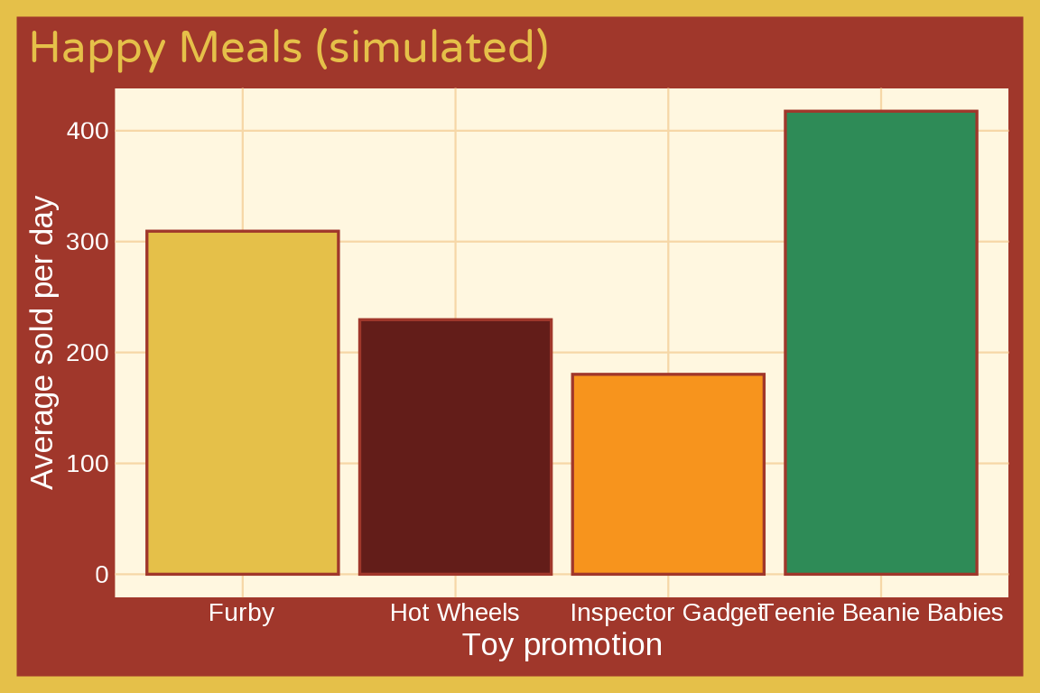
Hypercolor
theme_hypercolor(): heat changing magenta, orange, purple, and blue. Below we simulate monthly sales for two fads.
months <- seq(1990, 1995, by = 1 / 12)
fads <- data.frame(month = rep(months, 2),
                   fad = rep(c("Hypercolor", "Slap bracelets"), each = length(months)))
fads$sales <- ifelse(fads$fad == "Hypercolor",
                     4000 * dnorm(fads$month, 1991.5, 0.6),
                     3000 * dnorm(fads$month, 1990.8, 0.4)) / 12
ggplot(fads, aes(x = month, y = sales, fill = fad)) +
  geom_area(alpha = 0.8) +
  labs(title = "90s fads (simulated)", x = NULL, y = "Sales (thousands)", fill = NULL) +
  theme_hypercolor(base_size = 13)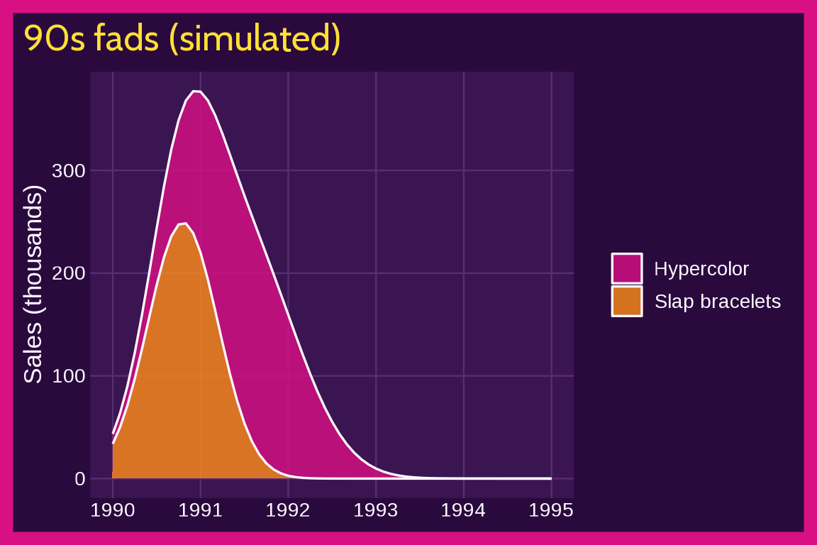
With mode = "light":
last_plot() + theme_hypercolor(base_size = 13, mode = "light")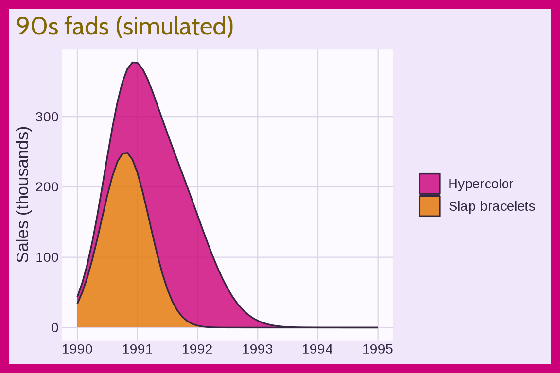
IBM Microdrive
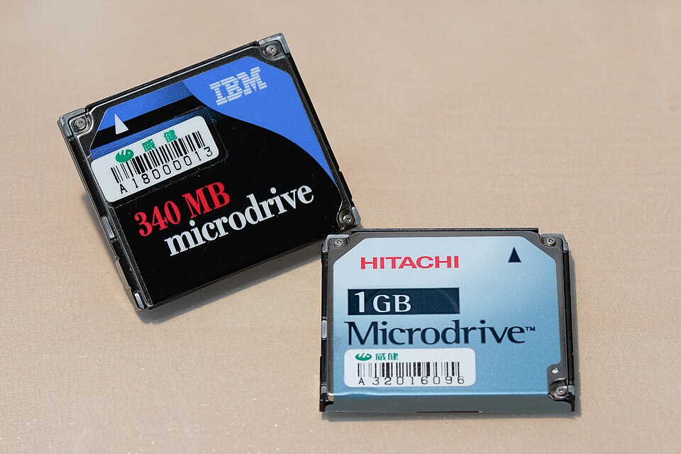
theme_microdrive() uses an IBM and a Hitachi Microdrive on a tan desk: a black frame, IBM blue, red, navy, and Hitachi sky blue marks, and a red Tinos title. Below we simulate photo file sizes from three digital cameras that wrote to a Microdrive.
set.seed(1999)
photos <- data.frame(camera = rep(c("2 MP", "3 MP", "4 MP"), each = 100))
photos$mb <- rlnorm(300, log(c("2 MP" = 0.9, "3 MP" = 1.4, "4 MP" = 2)[photos$camera]), 0.25)
ggplot(photos, aes(x = camera, y = mb, fill = camera)) +
  geom_boxplot(show.legend = FALSE) +
  labs(title = "Microdrive photos", caption = "Simulated data", x = NULL, y = "Photo size (MB)") +
  theme_microdrive(base_size = 13)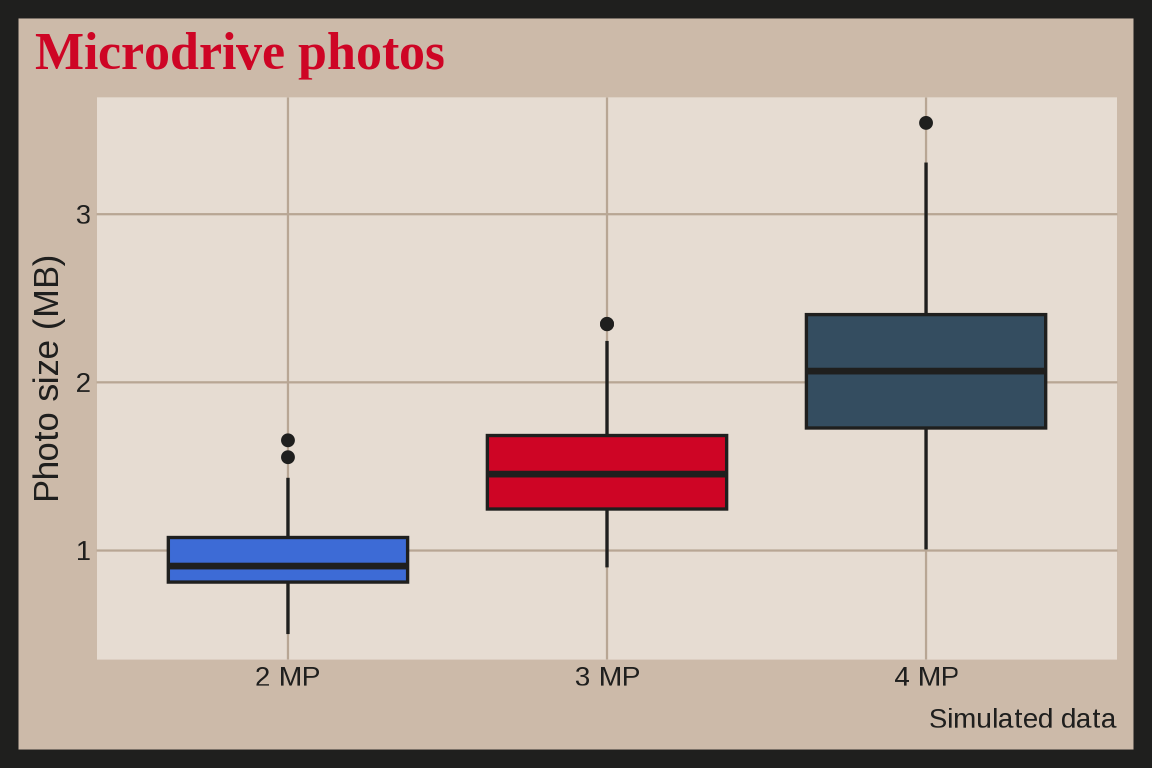
J2ME
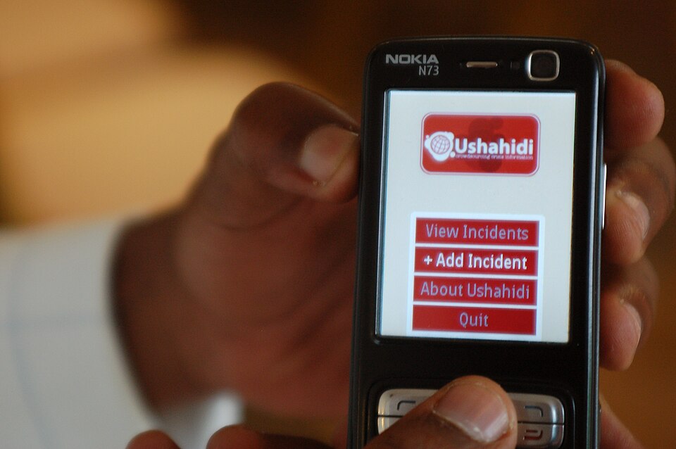
theme_j2me() uses a Nokia N73 running a J2ME app: a black phone background, a silver frame, a pale screen panel, Ushahidi red, tan, brown, and black marks, and an Archivo Narrow title. Below we simulate monthly downloads of four kinds of phone games.
set.seed(2003)
games <- expand.grid(month = 1:24, genre = c("Puzzle", "Racing", "Sports", "Arcade"))
games$downloads <- rpois(nrow(games), c(Puzzle = 60, Racing = 40, Sports = 30, Arcade = 20)[games$genre] * (1 + games$month / 12))
ggplot(games, aes(x = month, y = downloads, color = genre)) +
  geom_line(linewidth = 1) +
  labs(title = "J2ME game downloads", caption = "Simulated data", x = "Month", y = "Downloads (thousands)", color = NULL) +
  theme_j2me(base_size = 13)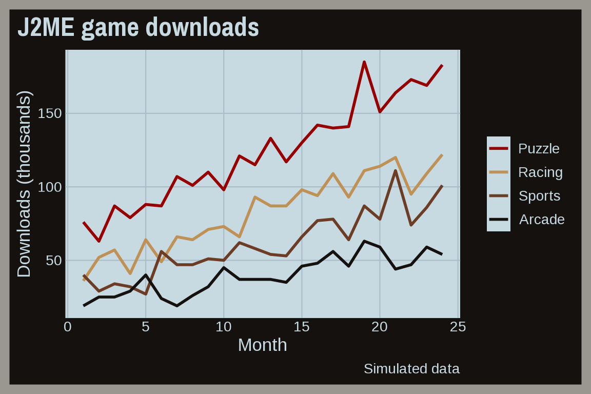
Java applets
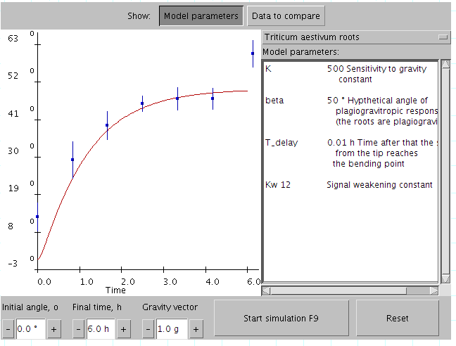
theme_javaapplet() uses a Java AWT applet window: a gray window background, a gray frame, a white panel, red, blue, purple, and gray marks, and a blue Noto Sans title. Below we simulate measurements with error bars and a fitted curve, like the applet in the screenshot.
set.seed(1995)
model <- data.frame(time = seq(0, 6, by = 0.1))
model$angle <- 48 * (1 - exp(-model$time / 1.2))
obs <- data.frame(time = seq(0, 6, by = 0.8))
obs$angle <- 48 * (1 - exp(-obs$time / 1.2)) + rnorm(nrow(obs), 0, 4)
ggplot(obs, aes(x = time, y = angle)) +
  geom_line(data = model, aes(color = "Model")) +
  geom_pointrange(aes(ymin = angle - 6, ymax = angle + 6, color = "Observed")) +
  labs(title = "Root bending angle", caption = "Simulated data", x = "Time (h)", y = "Angle (degrees)", color = NULL) +
  theme_javaapplet(base_size = 13)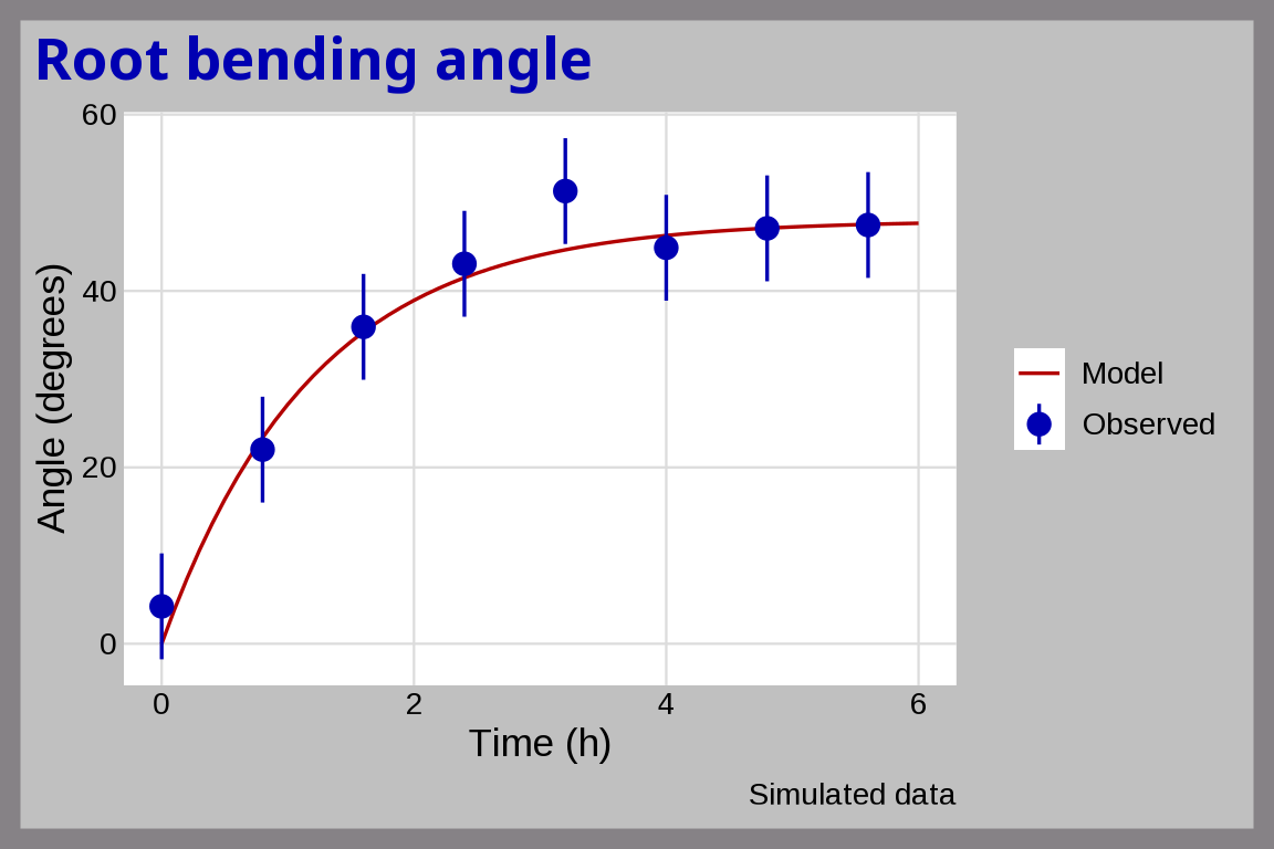
Jurassic Park
theme_jurassic() uses the Jurassic Park Post Office souvenir sheet: black, logo red, stamp yellow, and sunset orange. Below we simulate the total weight of the dinosaurs in each paddock.

set.seed(1993)
jp_paddocks <- data.frame(species = c("Brachiosaurus", "Triceratops", "Tyrannosaurus"),
  total_tons = c(sum(rnorm(3, 40, 5)), sum(rnorm(5, 9, 1.2)), sum(rnorm(2, 8, 1))))
ggplot(jp_paddocks, aes(x = species, y = total_tons, fill = species)) +
  geom_col(show.legend = FALSE) +
  labs(title = "Jurassic Park (simulated)", x = "Paddock", y = "Total weight (tons)") +
  theme_jurassic(base_size = 13)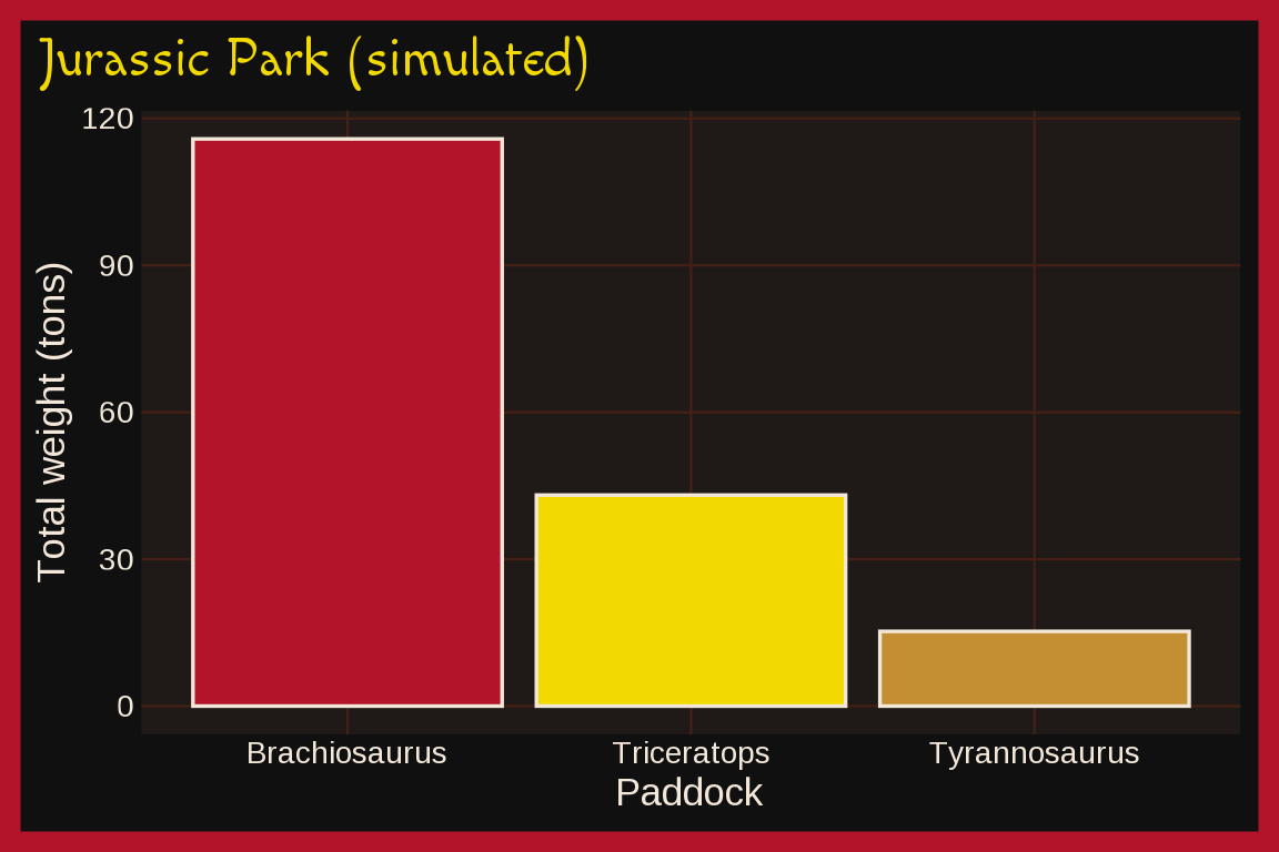
With mode = "light":
last_plot() + theme_jurassic(base_size = 13, mode = "light")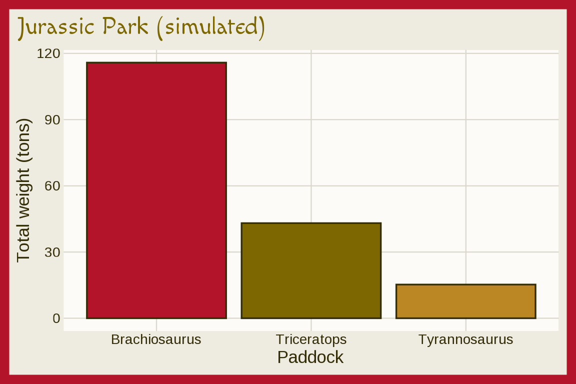
Koosh ball
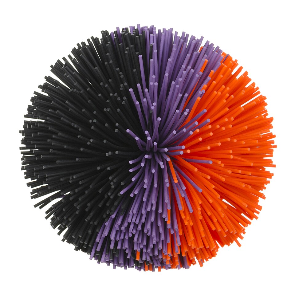
theme_koosh() uses a tri color Koosh ball: a white background, an orange frame, orange, purple, and black marks, and an Varela Round title. Below we simulate the styles of 200 Koosh balls sold at a toy store.
set.seed(1993)
koosh_balls <- data.frame(style = factor(sample(c("Tri color", "Rainbow", "Neon", "Glow"),
  200, replace = TRUE, prob = c(1/2, 1/4, 1/8, 1/8)),
  levels = c("Tri color", "Rainbow", "Neon", "Glow")))
ggplot(koosh_balls, aes(x = style, fill = style)) +
  geom_bar(show.legend = FALSE) +
  labs(title = "Koosh balls", caption = "Simulated data", x = NULL, y = "Sold") +
  theme_koosh(base_size = 13)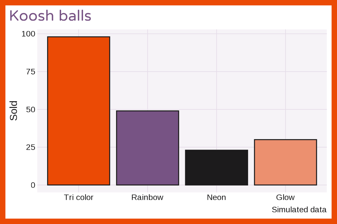
Netscape
theme_netscape(): the Netscape Navigator logo, with a night sky background, teal, aurora green, sea glass, and deep teal marks, and a Tinos title. Below we simulate dial up speeds for three modems.

set.seed(1996)
modem <- sample(c("14.4k", "28.8k", "56k"), 600, replace = TRUE, prob = c(0.25, 0.45, 0.30))
speeds <- data.frame(modem = modem,
  kbps = rnorm(600, c(`14.4k` = 13, `28.8k` = 26, `56k` = 44)[modem], c(`14.4k` = 1.2, `28.8k` = 2.5, `56k` = 5)[modem]))
ggplot(speeds, aes(x = kbps, after_stat(count), fill = modem)) +
  geom_density(position = "fill") +
  labs(title = "Dial up speeds (simulated)", x = "Speed (kbps)", fill = "Modem") +
  theme_netscape(base_size = 13)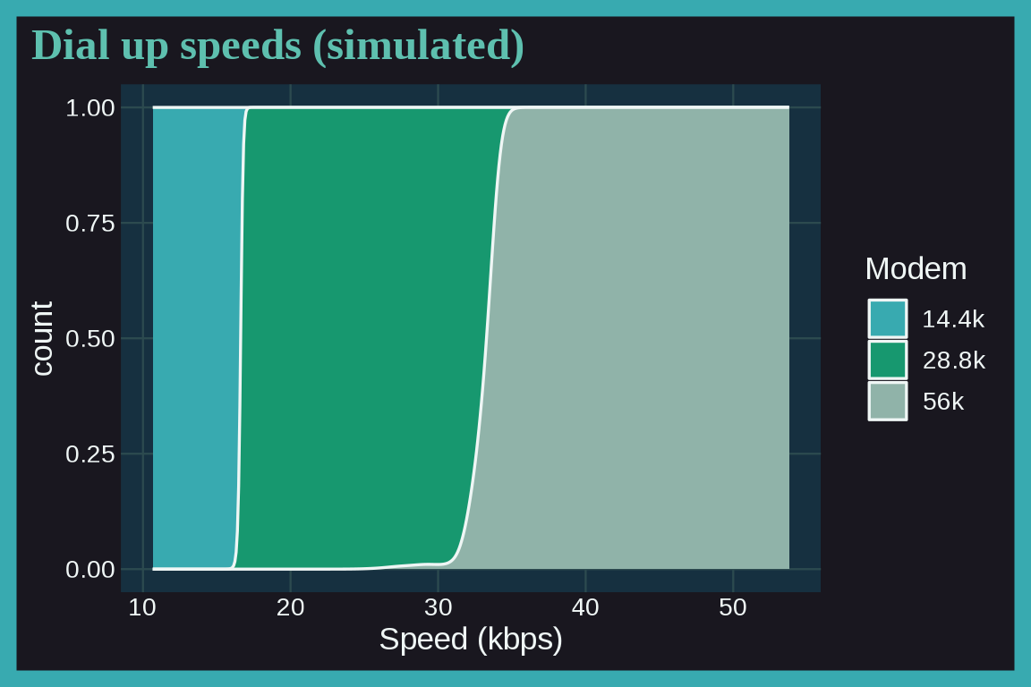
With mode = "light":
last_plot() + theme_netscape(base_size = 13, mode = "light")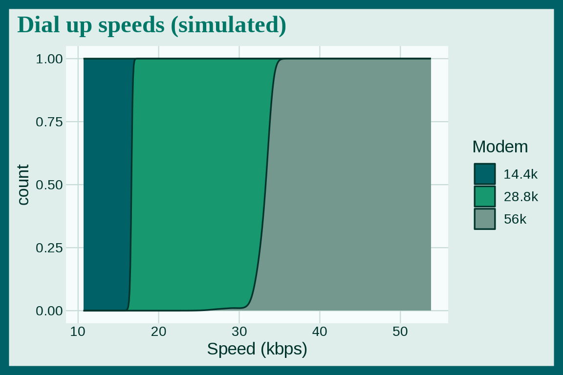
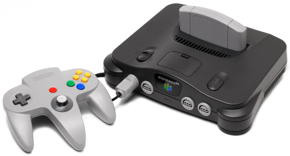
Nintendo 64
theme_n64() uses controller gray and the four logo colors. Below we simulate 200 Mario Kart 64 lap times from a heavy tailed t distribution.
set.seed(64)
mario_kart_laps <- data.frame(seconds = 45 + 2 * rt(n = 200, df = 3))
ggplot(mario_kart_laps, aes(x = "", y = seconds)) +
  geom_boxplot() +
  labs(title = "Mario Kart 64 (simulated)",
       x = NULL, y = "Lap time (seconds)") +
  theme_n64(base_size = 13)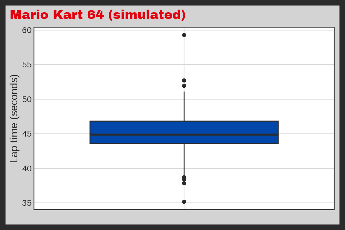
Novell NetWare
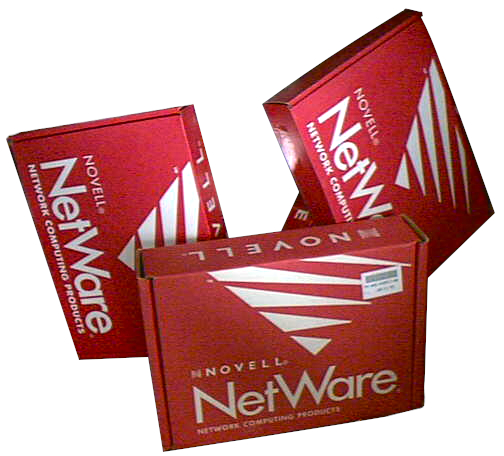
theme_netware() uses three NetWare 2.0 boxes: a pale blush background with dark ink text, a NetWare red frame and title, maroon, red, rose, and blush marks, and a Cabin title. Below we simulate the file servers running each NetWare version from 1990 to 1998.
set.seed(1990)
servers <- expand.grid(year = 1990:1998, version = c("2.x", "3.x", "4.x"))
servers$peak <- c("2.x" = 1990, "3.x" = 1994, "4.x" = 1998)[servers$version]
servers$n <- rpois(nrow(servers), 400 * exp(-((servers$year - servers$peak) / 2.5)^2))
ggplot(servers, aes(x = year, y = n, fill = version)) +
  geom_col() +
  labs(title = "NetWare servers", caption = "Simulated data", x = NULL, y = "Servers", fill = "Version") +
  theme_netware(base_size = 13)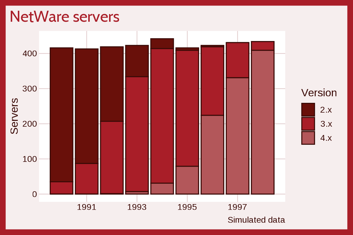
OK Soda
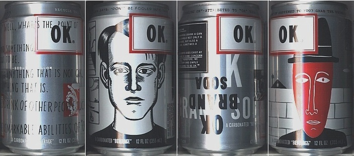
theme_oksoda() uses the gray comic book cans Coca-Cola sold from 1993 to 1995: brushed silver, black ink, OK red bars, slate and brick accents, and an OK red Cousine title. Below we simulate one day of sales at 300 test market stores from a normal distribution.
set.seed(1014)
ok_soda_sales <- data.frame(
  cans = round(rnorm(n = 300, mean = 45, sd = 12))
)
ggplot(ok_soda_sales, aes(x = cans)) +
  geom_histogram(bins = 30) +
  labs(title = "OK Soda", caption = "Simulated data",
       subtitle = "Cans sold per store in one day",
       x = "Cans sold") +
  theme_oksoda(base_size = 13)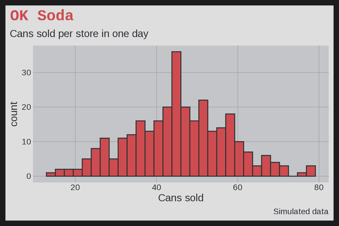
Orbitz
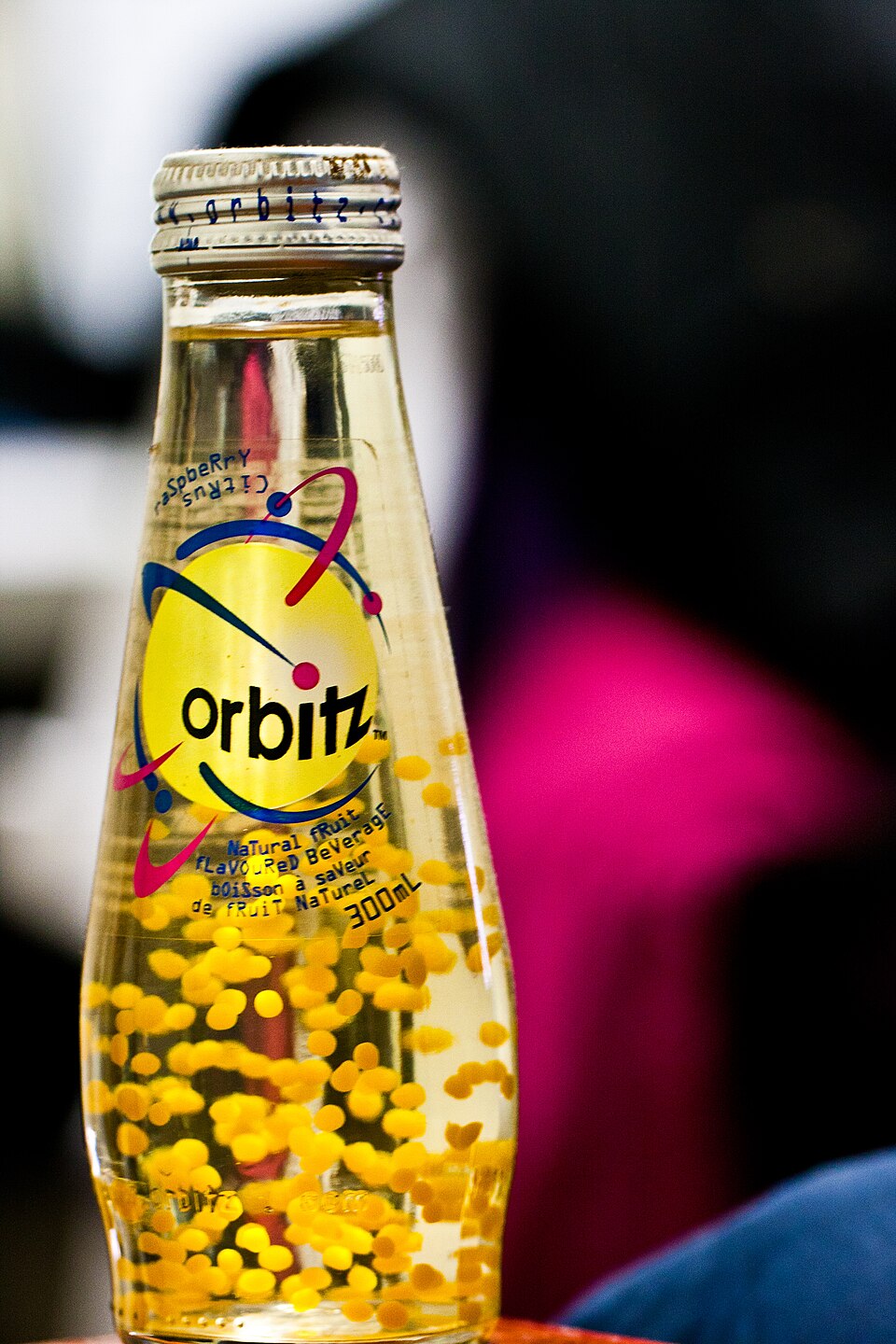
theme_orbitz() uses a bottle of Orbitz, the 1997 drink with floating gel balls: a black background, a gold frame, gold and magenta marks, and a Permanent Marker title. Below we compare the share of kids buying Orbitz and Surge each week after Orbitz arrived.
p_surge <- 0.8 * plogis(-2 + 0.6 * (0:6))
drinks <- data.frame(week = factor(rep(1:7, 2)),
  choice = factor(rep(c("Surge", "Orbitz"), each = 7), levels = c("Surge", "Orbitz")),
  share = c(p_surge, -(0.8 - p_surge)))
ggplot(drinks, aes(x = week, y = share, fill = choice)) +
  geom_col(width = 0.5) +
  labs(title = "Orbitz vs. Surge", caption = "Simulated data",
       x = "Week", y = "Share of kids", fill = NULL) +
  theme_orbitz(base_size = 13)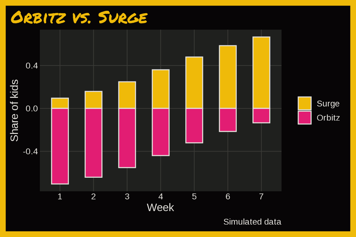
With mode = "light":
last_plot() + theme_orbitz(base_size = 13, mode = "light")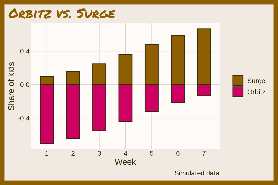
Oregon Trail
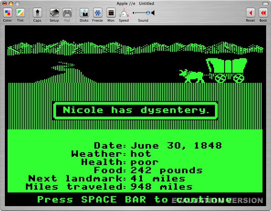
theme_oregontrail(): The Oregon Trail running in an Apple II emulator, with a gray window frame, a black screen, and three shades of phosphor green. Below we simulate days to reach Oregon from a log normal distribution.
set.seed(1985)
trips <- data.frame(profession = rep(c("Banker", "Carpenter", "Farmer"), each = 100))
trips$days <- rlnorm(300, log(c(Banker = 140, Carpenter = 155, Farmer = 170)[trips$profession]), 0.2)
ggplot(trips, aes(x = profession, y = days, fill = profession)) +
  geom_boxplot(alpha = 2/3, show.legend = FALSE) +
  labs(title = "The Oregon Trail (simulated)", x = NULL, y = "Days") +
  theme_oregontrail(base_size = 13)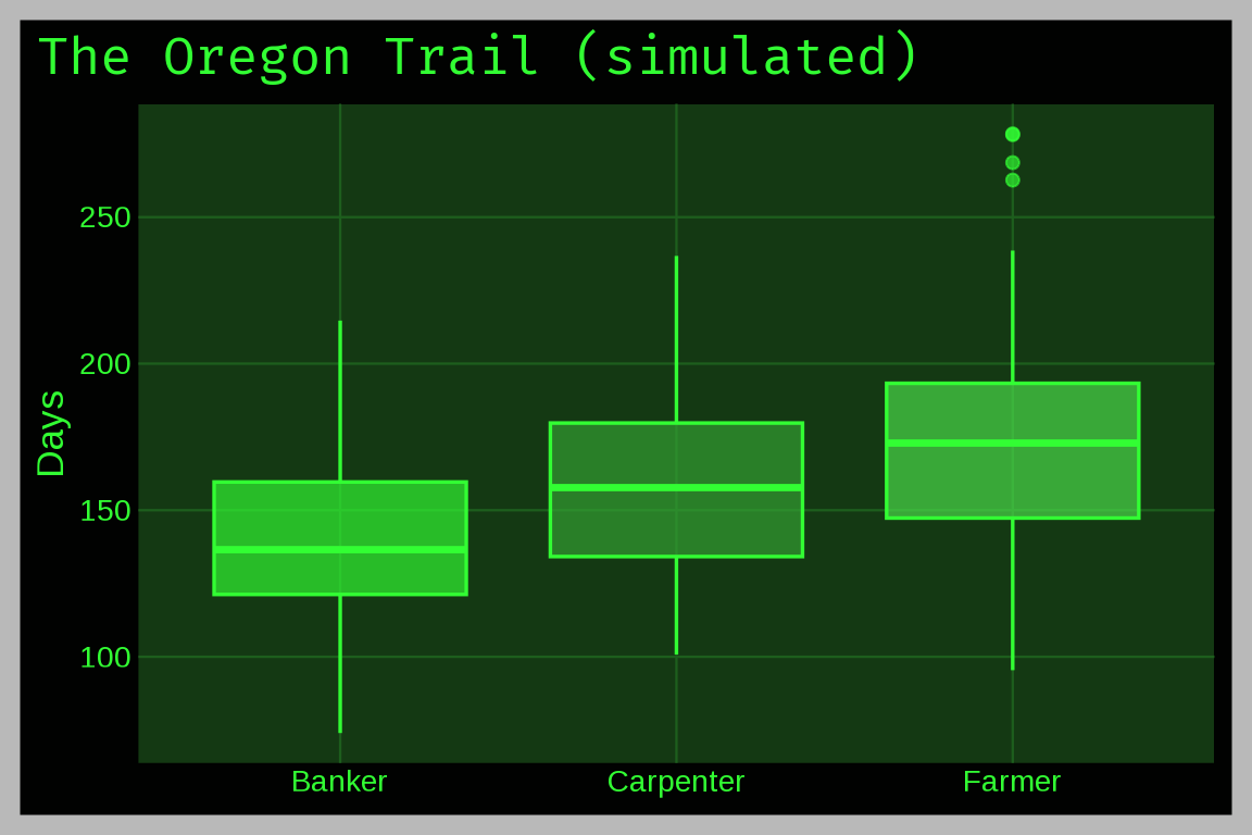
With mode = "light":
last_plot() + theme_oregontrail(base_size = 13, mode = "light")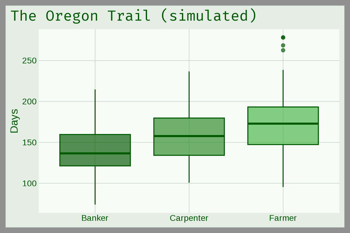
Palm Pilot
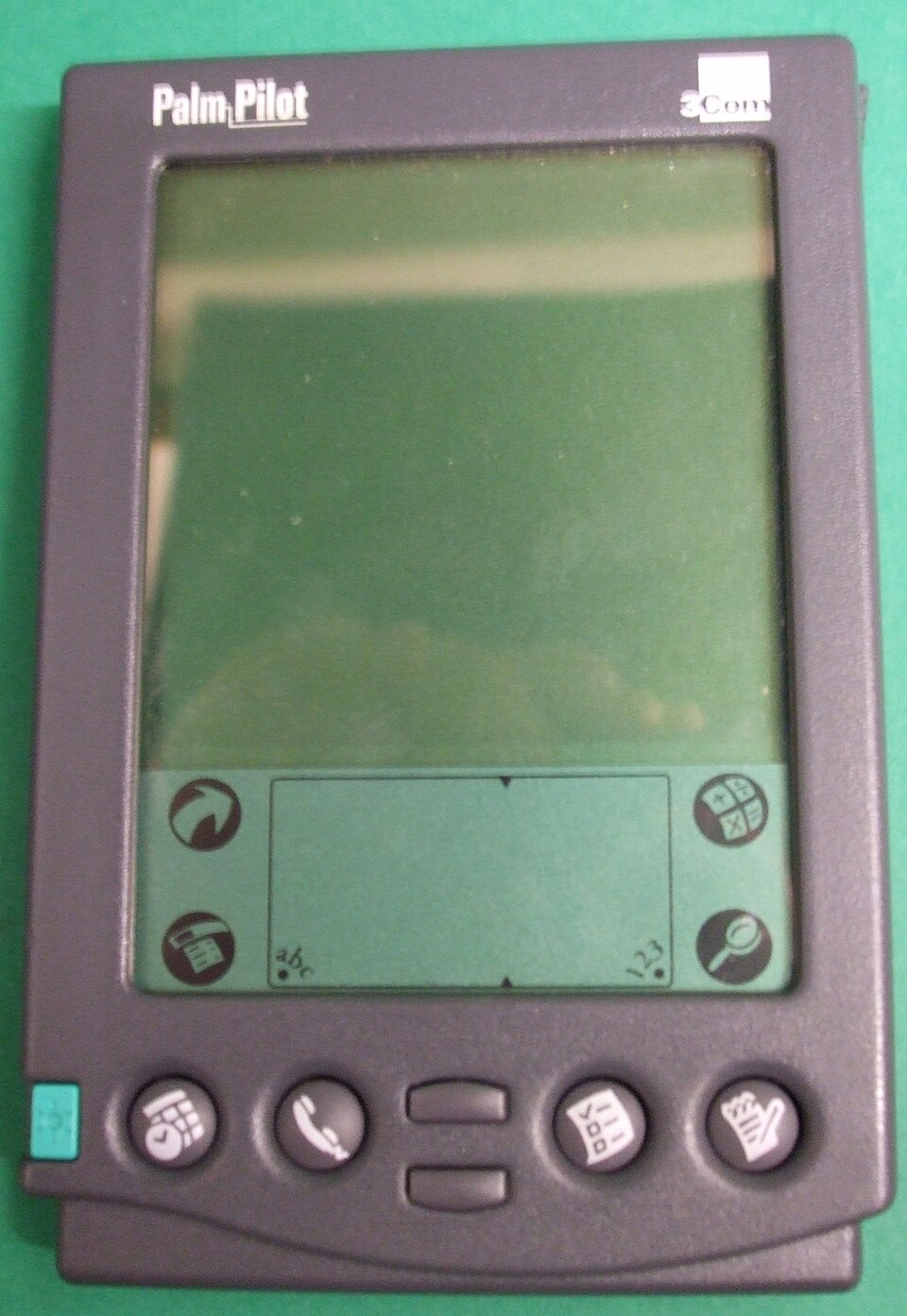
theme_palmpilot() uses a PalmPilot Professional: a charcoal case background, a HotSync teal frame, a green LCD panel, ink, LCD green, plum, and teal marks, and a white Jost title. Below we simulate how Graffiti accuracy improves over a user’s first ten weeks.
set.seed(1997)
graffiti <- data.frame(week = runif(200, 0, 10))
graffiti$accuracy <- pmin(100, 98 - 30 * exp(-graffiti$week / 2) + rnorm(200, 0, 3))
ggplot(graffiti, aes(x = week, y = accuracy)) +
  geom_point(alpha = 1 / 2) +
  geom_smooth(method = "loess", formula = y ~ x, se = FALSE) +
  labs(title = "Learning Graffiti", caption = "Simulated data", x = "Weeks of use", y = "Characters recognized (%)") +
  theme_palmpilot(base_size = 13)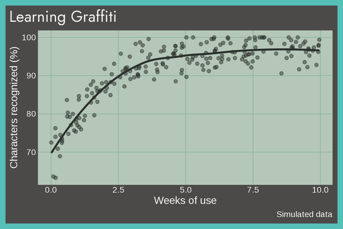
Pogs
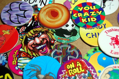
theme_pogs() uses a cardboard background and the red, sky blue, yellow, teal, purple, and rust milk cap prints. Below we simulate a collection of 100 Pogs.
set.seed(1993)
pogs <- data.frame(type = sample(c("Milk caps", "Printed pogs", "Holographic", "Slammers"),
  100, replace = TRUE, prob = c(0.45, 0.30, 0.15, 0.10)))
ggplot(pogs, aes(x = type, fill = type)) +
  geom_bar(show.legend = FALSE) +
  labs(title = "A Pogs collection (simulated)", x = NULL, y = "Pieces") +
  theme_pogs(base_size = 13)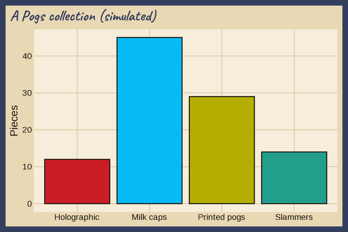
Power Rangers
theme_powerrangers(): the six Ranger suits on light gray. Below we simulate putties defeated by each Ranger.

set.seed(1993)
fights <- data.frame(ranger = factor(rep(c("Red", "Blue", "Yellow", "Pink", "Black"), each = 20), levels = c("Red", "Blue", "Yellow", "Pink", "Black")), minutes = rgamma(100, 4, 1))
fights$putties <- rpois(100, 1.6 * fights$minutes)
ggplot(fights, aes(x = minutes, y = putties, fill = ranger)) +
  geom_point(shape = 21, size = 3, color = "#000000") +
  labs(title = "Power Rangers", caption = "Simulated data", x = "Fight minutes", y = "Putties defeated", fill = NULL) +
  theme_powerrangers(base_size = 13)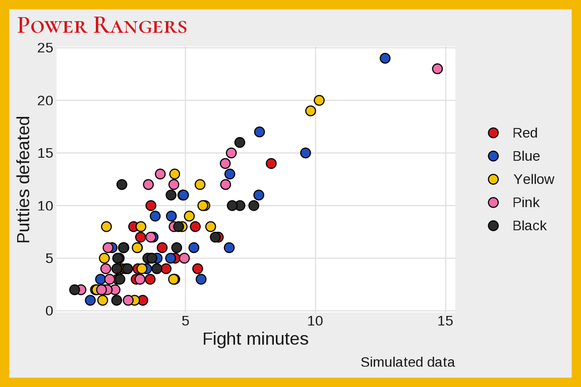
Saved by the Bell
theme_savedbythebell(): the logo’s sky blue, pink, yellow, and orange on black. Below we simulate fall and spring quiz averages for three students.

set.seed(1989)
grades <- data.frame(student = rep(c("Zack", "Kelly", "Screech"), 2),
                     semester = rep(c("Fall", "Spring"), each = 3))
grades$score <- c(70, 82, 93, 80, 82, 95) + rnorm(6, 0, 2)
ggplot(grades, aes(x = semester, y = score, group = student, color = student)) +
  geom_line(linewidth = 2) +
  geom_point(size = 4) +
  labs(title = "Bayside quizzes (simulated)", x = NULL, y = "Average score", color = NULL) +
  theme_savedbythebell(base_size = 13)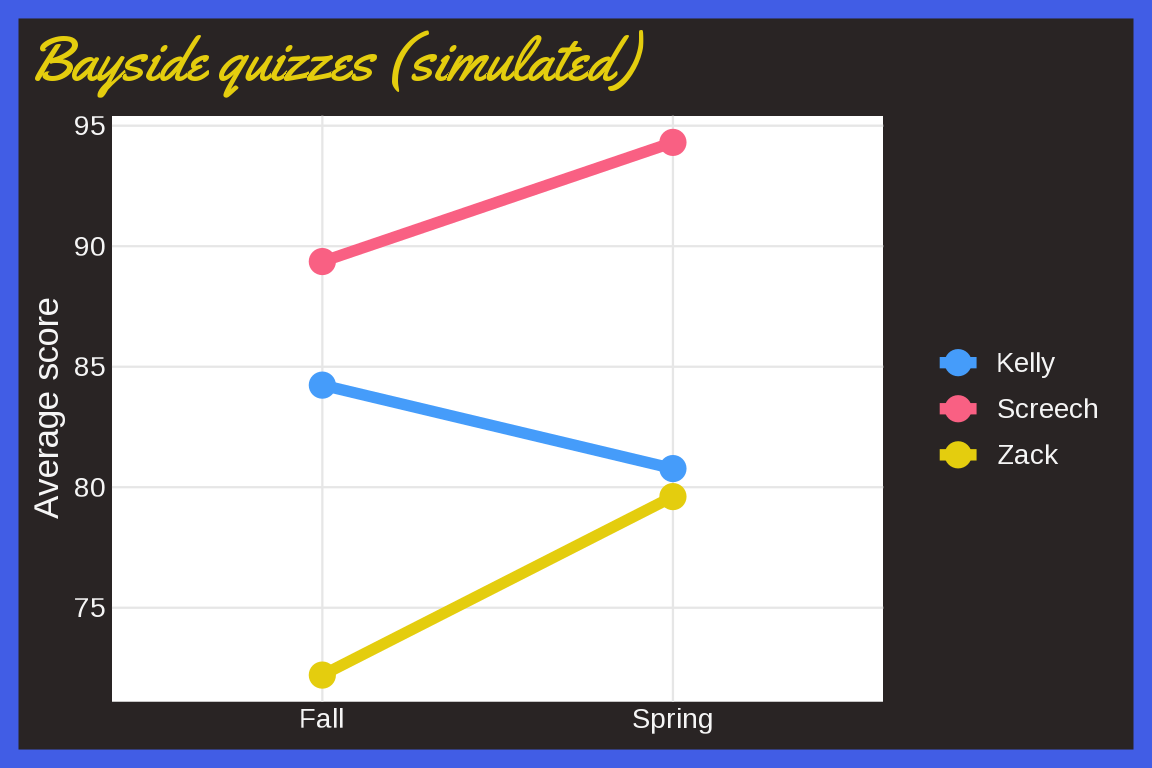
Seinfeld
theme_seinfeld(): the Seinfeld logo, with a yellow frame and a red title on the black drop shadow. The light version puts the plot on the yellow oval. Below we simulate laughs and viewers for 60 episodes.

set.seed(1989)
eps <- data.frame(kramer = rgamma(60, 6, 1.5), viewers = rlnorm(60, log(20), 0.3))
eps$laughs <- 2 + 0.3 * eps$kramer + rnorm(60, 0, 0.5)
ggplot(eps, aes(x = kramer, y = laughs, size = viewers)) +
  geom_point(alpha = 1 / 2) +
  labs(title = "Seinfeld episodes", caption = "Simulated data", x = "Kramer minutes", y = "Laughs per minute", size = "Viewers") +
  theme_seinfeld(base_size = 13)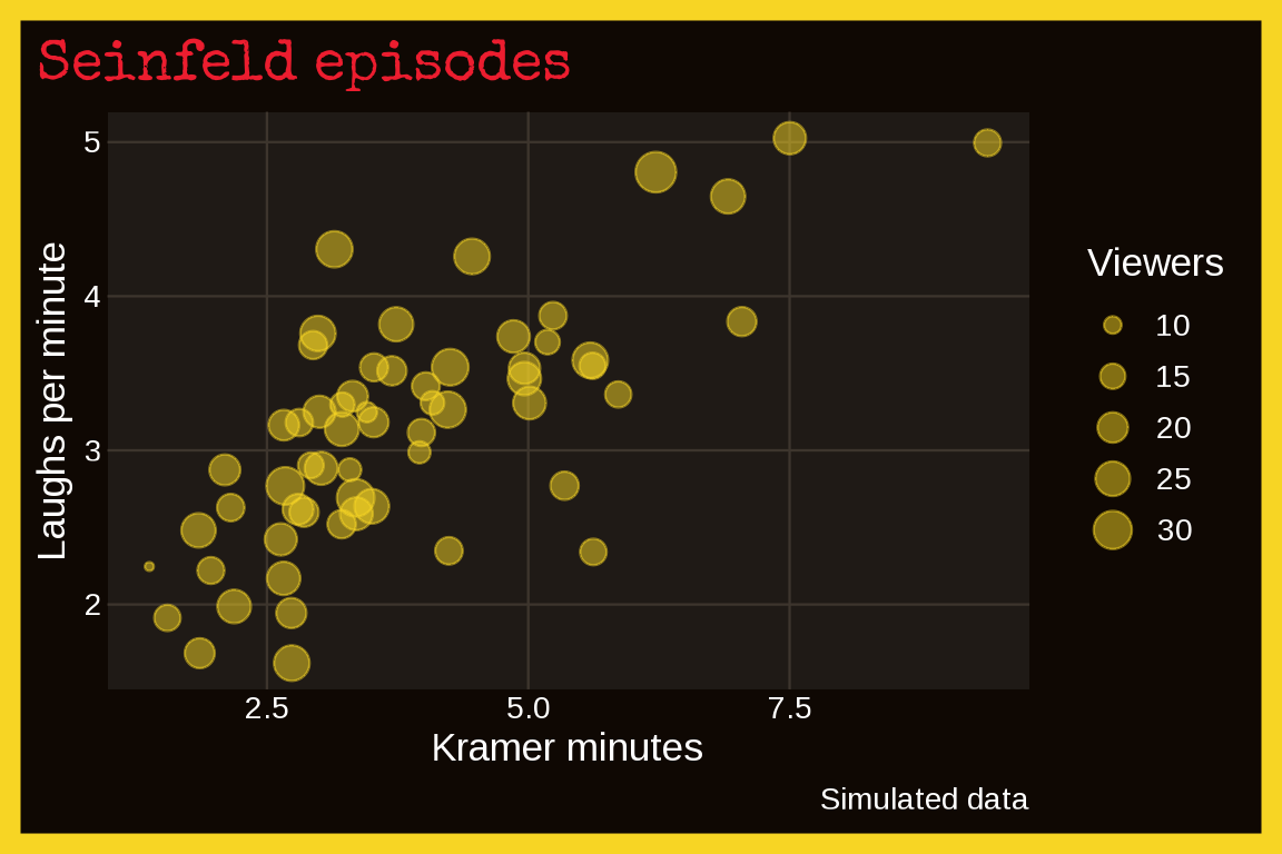
With mode = "light":
last_plot() + theme_seinfeld(base_size = 13, mode = "light")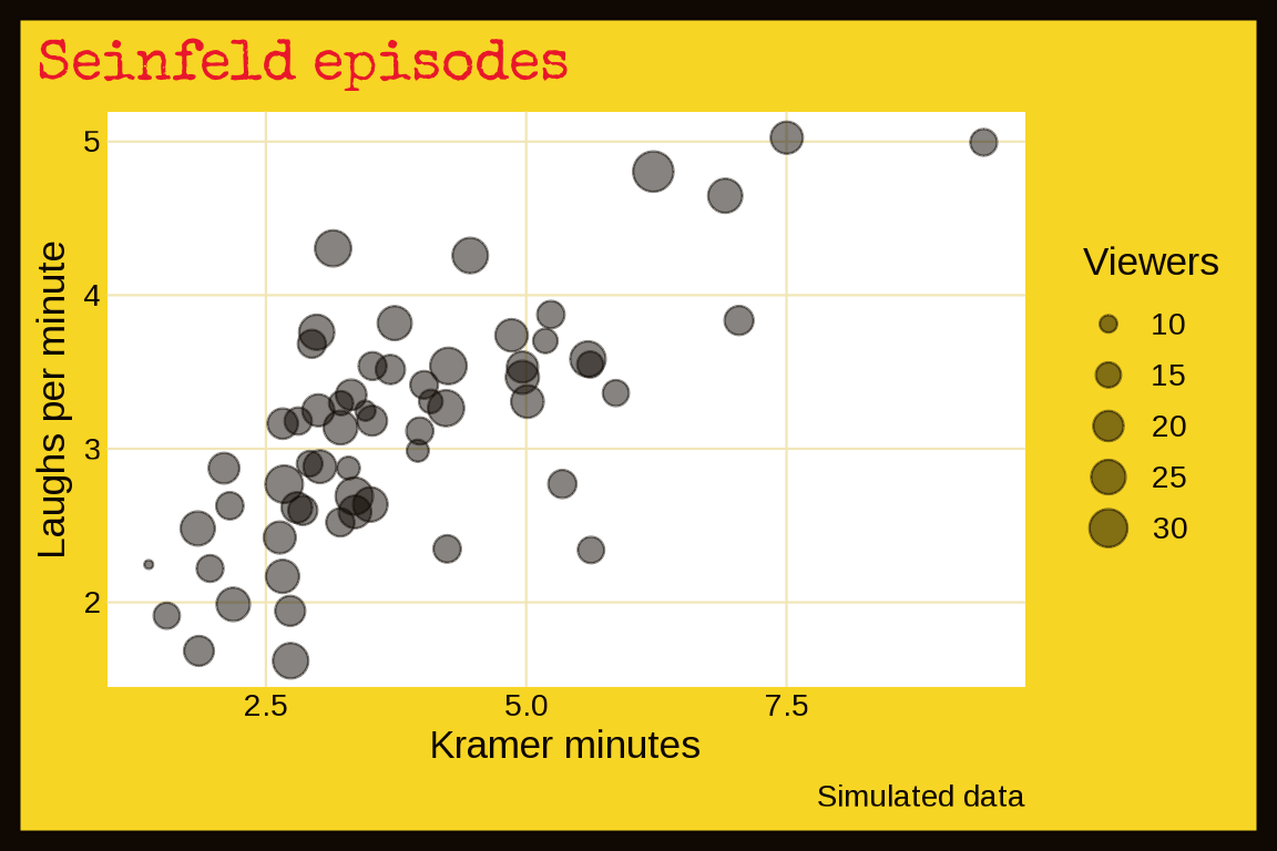
SNICK
theme_snick(): Nickelodeon orange and slime green on a night purple sky. Below we simulate 20 weeks of ratings for three nights.

set.seed(1992)
nights <- expand.grid(week = 1:20, night = c("Fri", "Sat", "Sun"))
nights$rating <- c(Fri = 2.8, Sat = 4.2, Sun = 3.0)[as.character(nights$night)] + rnorm(60, 0, 0.3)
ggplot(nights, aes(x = week, y = rating, color = night)) +
  geom_line(linewidth = 1) +
  labs(title = "SNICK ratings (simulated)", x = "Week", y = "Rating", color = NULL) +
  theme_snick(base_size = 13)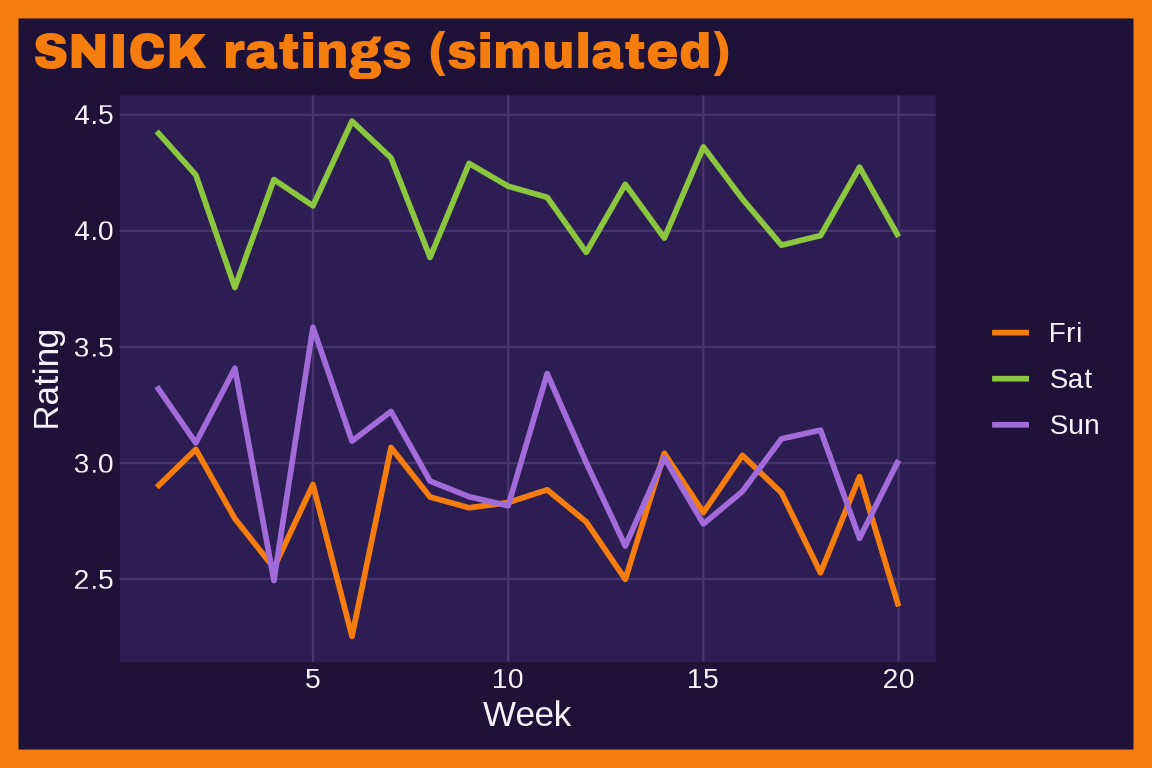
With mode = "light":
last_plot() + theme_snick(base_size = 13, mode = "light")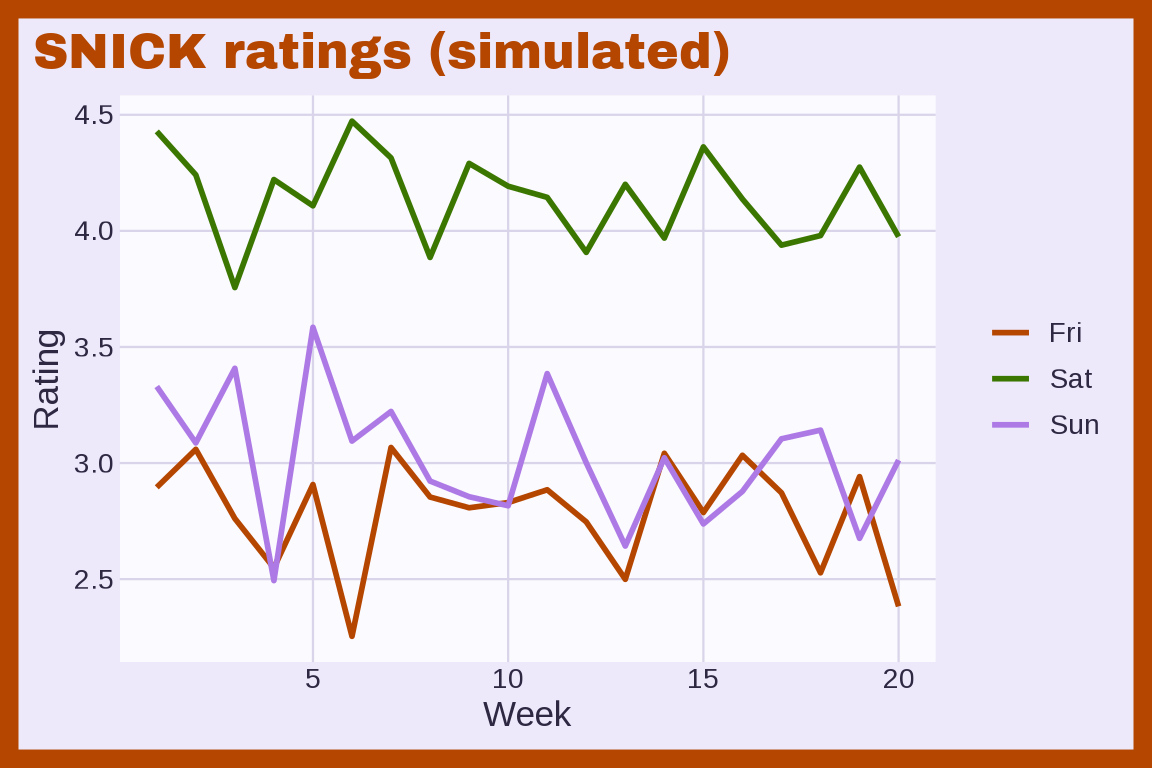
Sony Walkman
theme_walkman() uses the Sports Walkman: a sports yellow body, blue buttons, a charcoal display, and an orange SPORTS label. Below we simulate median battery life for three models and two battery types.
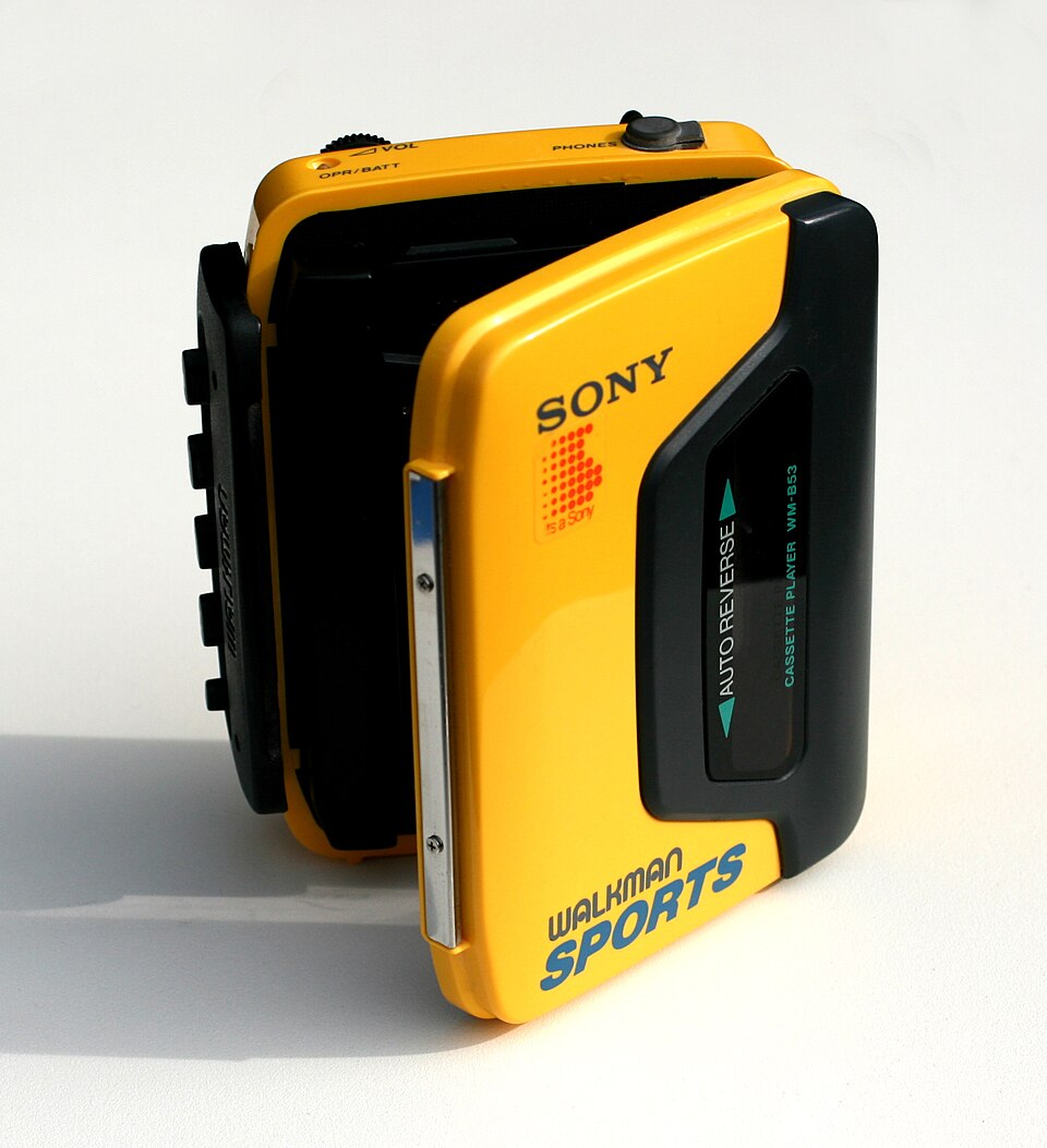
set.seed(1979)
walkman <- data.frame(model = rep(c("WM-2", "WM-F45 Sports", "WM-EX194 Mega Bass"), times = 2),
  battery = rep(c("Alkaline", "Rechargeable"), each = 3), hours = c(10, 16, 22, 7, 12, 17) + rnorm(6, 0, 0.5))
ggplot(walkman, aes(x = hours, y = model)) +
  geom_line(aes(group = model)) +
  geom_point(aes(color = battery), size = 3) +
  labs(title = "Sony Walkman (simulated)", x = "Median battery life (hours)", y = NULL, color = "Battery") +
  theme_walkman(base_size = 13)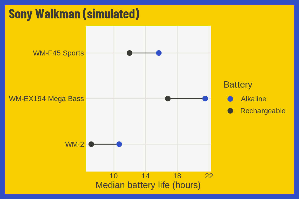
Squeezit
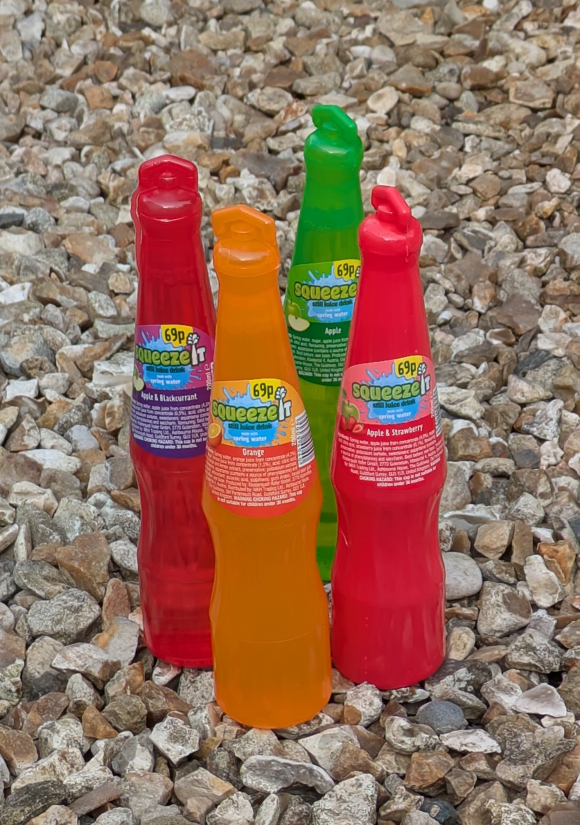
theme_squeezit() uses Squeezit bottles standing in gravel: a gravel background, a red frame and title, red, orange, green, pink, blue, and gold marks, and a Marcellus title. Below we use a gamma distribution to simulate the seconds it took to finish three flavors.
set.seed(1998)
bottles <- data.frame(flavor = factor(rep(c("Cherry", "Orange", "Green punch"), each = 60),
  levels = c("Cherry", "Orange", "Green punch")))
bottles$seconds <- rgamma(180, shape = 2.5,
  scale = c(Cherry = 12, Orange = 18, `Green punch` = 22)[as.character(bottles$flavor)] / 2.5)
ggplot(bottles, aes(x = seconds, fill = flavor)) +
  geom_density(alpha = 2/3) +
  labs(title = "Squeezit", caption = "Simulated data",
       x = "Seconds to finish", fill = "Flavor") +
  theme_squeezit(base_size = 13)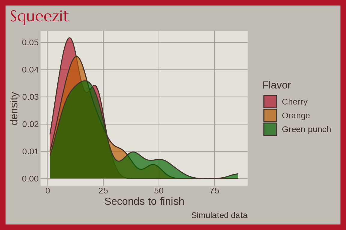
Super Soaker
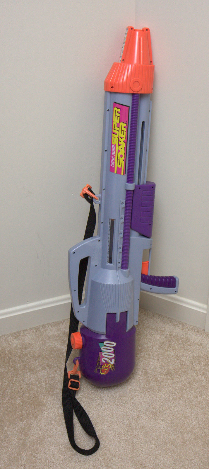
theme_supersoaker(): neon orange plastic, water blue, and neon green. Below we simulate Super Soaker ranges for two models.
set.seed(1990)
shots <- data.frame(model = rep(c("SS 50", "CPS 2000"), each = 200))
shots$feet <- rnorm(400, ifelse(shots$model == "SS 50", 25, 45), ifelse(shots$model == "SS 50", 3, 5.4))
ggplot(shots, aes(x = feet, color = model)) +
  geom_freqpoly(binwidth = 2, linewidth = 1) +
  labs(title = "Super Soaker range (simulated)", x = "Range (feet)", color = "Model") +
  theme_supersoaker(base_size = 13)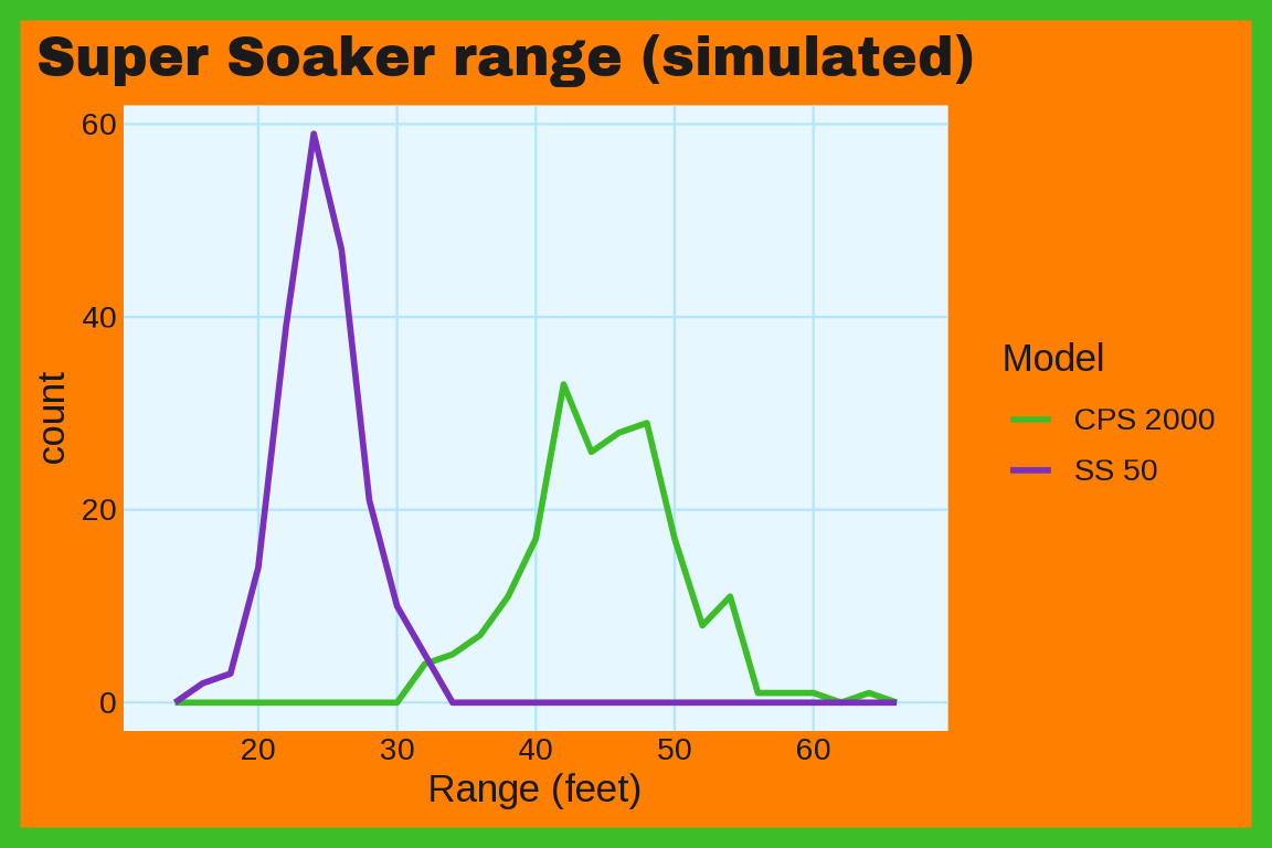
Surge
theme_surge(): Surge green on black, with a dark to bright green continuous scale. Below we simulate cans of Surge and hours of video games.
set.seed(1996)
teens <- data.frame(cans = rgamma(2000, 2, 0.5))
teens$hours <- 3 + 1.5 * teens$cans + rnorm(2000, 0, 3)
ggplot(teens, aes(x = cans, y = hours)) +
  geom_bin2d(bins = 20) +
  labs(title = "Surge and video games", caption = "Simulated data", x = "Cans per week", y = "Gaming hours") +
  theme_surge(base_size = 13)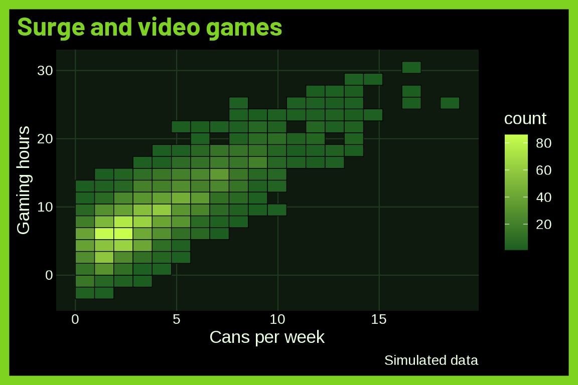
With mode = "light":
last_plot() + theme_surge(base_size = 13, mode = "light")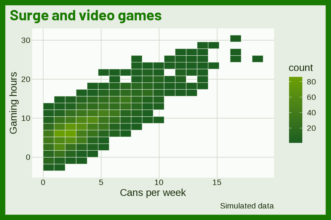
Talkboy
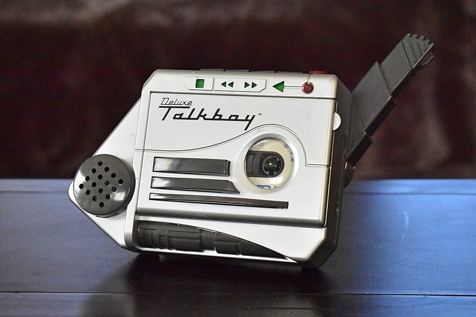
theme_talkboy() uses the Deluxe Talkboy from Home Alone 2 sitting on a walnut table: a silver panel, button blue marks, and a Kaushan Script title. Below we simulate the length of 300 recorded messages from a right skewed gamma distribution.
set.seed(1999)
talkboy_clips <- data.frame(
  seconds = round(rgamma(n = 300, shape = 4, rate = 0.5), 1)
)
ggplot(talkboy_clips, aes(x = seconds)) +
  geom_freqpoly(bins = 30) +
  labs(title = "Talkboy", caption = "Simulated data",
       subtitle = "Length of 300 recorded messages",
       x = "Message length (seconds)") +
  theme_talkboy(base_size = 13)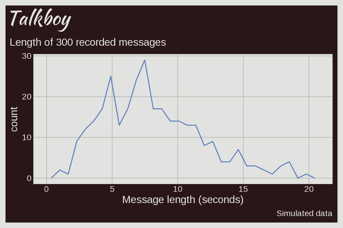
Tamagotchi
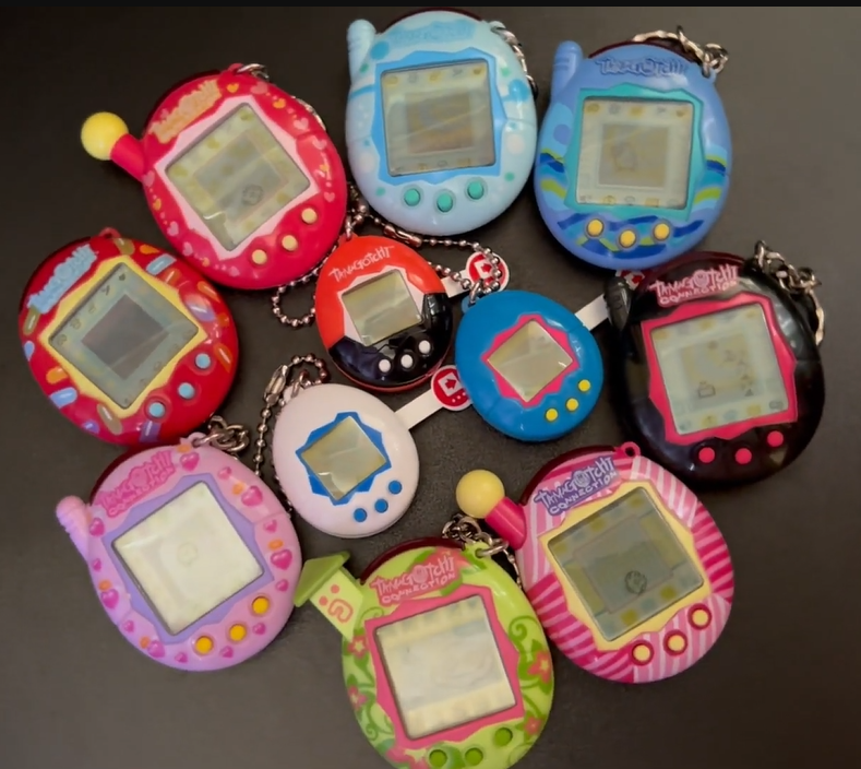
theme_tamagotchi(): a lilac egg shell and a gray green LCD screen. Below we simulate Tamagotchi lifespans from a Weibull distribution.
set.seed(1997)
pets <- data.frame(care = rep(c("Neglected", "Pampered"), each = 150))
pets$days <- rweibull(300, shape = 2.2, scale = ifelse(pets$care == "Neglected", 6, 21))
ggplot(pets, aes(x = days, fill = care)) +
  geom_histogram(alpha = 2/3, position = "identity", bins = 40) +
  labs(title = "Tamagotchi lifespans (simulated)", x = "Days", fill = "Care") +
  theme_tamagotchi(base_size = 13)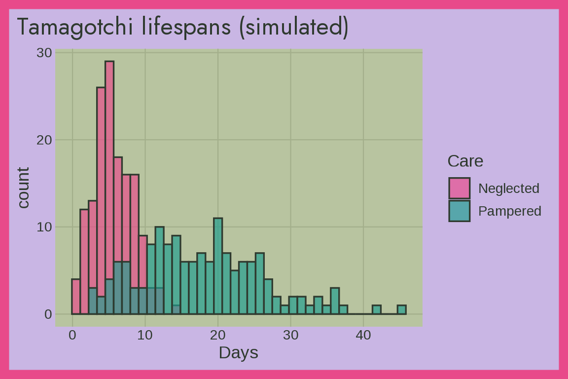
Tetris
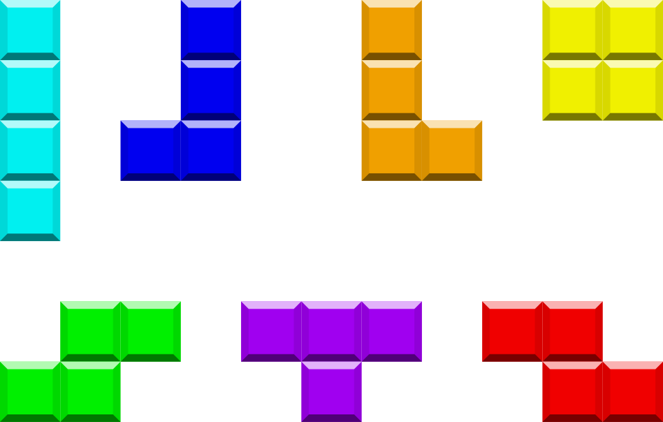
theme_tetris(): a black well and the seven tetromino colors. Below we simulate lines cleared from a negative binomial distribution.
set.seed(1989)
games <- data.frame(player = rep(c("Casual", "Expert"), each = 80))
games$lines <- rnbinom(160, size = 5, mu = ifelse(games$player == "Casual", 25, 120))
ggplot(games, aes(x = player, y = lines, color = player)) +
  geom_jitter(width = 0.2, show.legend = FALSE) +
  labs(title = "Tetris (simulated)", x = NULL, y = "Lines cleared") +
  theme_tetris(base_size = 13)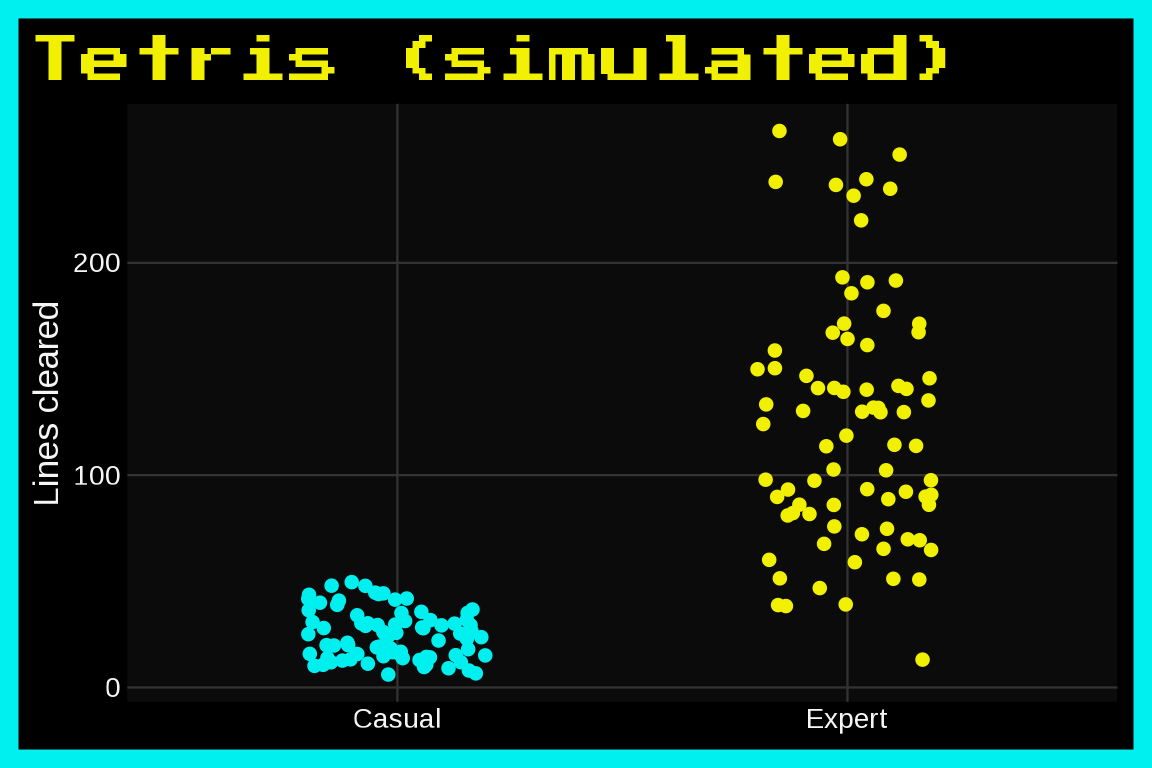
With mode = "light":
last_plot() + theme_tetris(base_size = 13, mode = "light")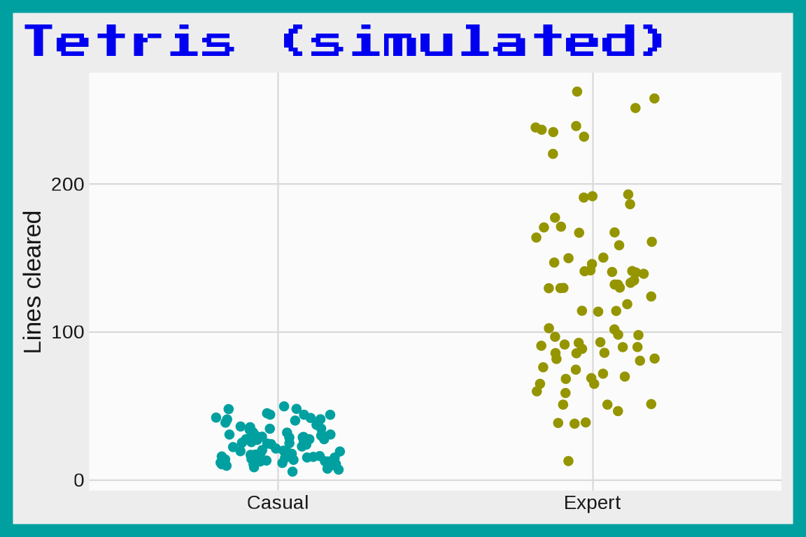
Tiger R-Zone
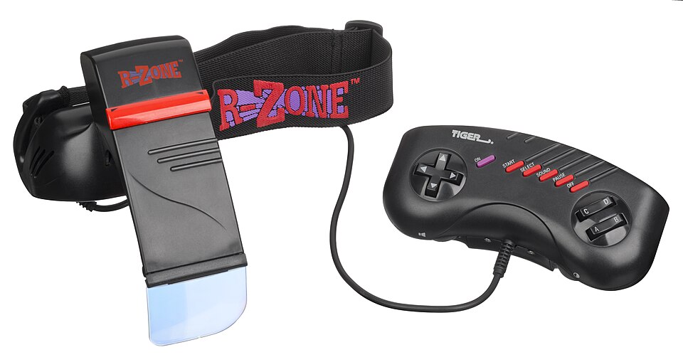
theme_rzone() uses Tiger’s 1995 R-Zone headset: black plastic, a red frame and title, red LCD, purple, and pink marks, pale blue visor text, and an Archivo Narrow title. Below we simulate the seconds 100 players needed to clear the first level on two tries.
set.seed(1993)
tries <- data.frame(try = rep(c("First", "Second"), each = 100))
tries$seconds <- rlnorm(200, log(ifelse(tries$try == "First", 40, 20)), 0.5)
ggplot(tries, aes(x = seconds, y = try, fill = try)) +
  geom_boxplot(width = 0.3, show.legend = FALSE) +
  labs(title = "Tiger R-Zone", caption = "Simulated data",
       x = "Seconds to clear the first level", y = NULL) +
  theme_rzone(base_size = 13)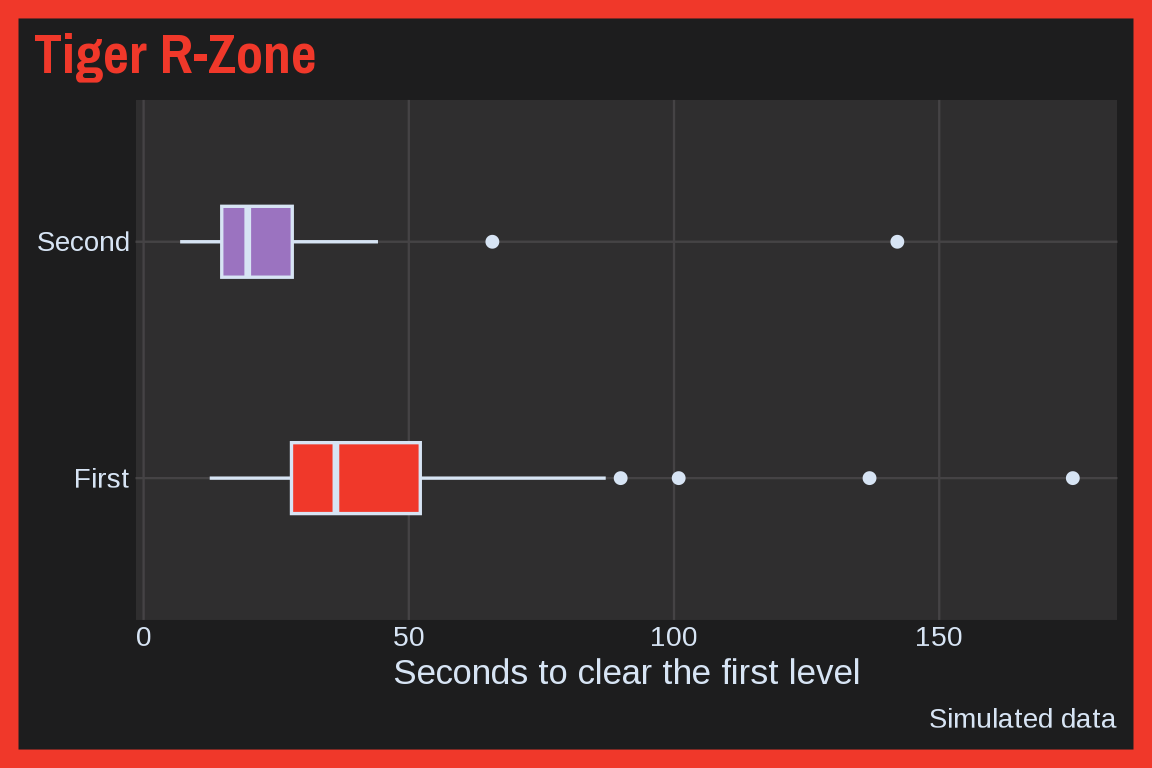
With mode = "light":
last_plot() + theme_rzone(base_size = 13, mode = "light")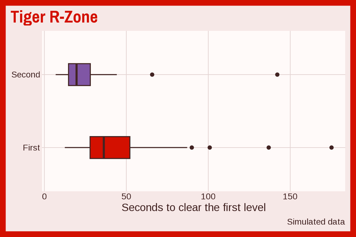
Titanic
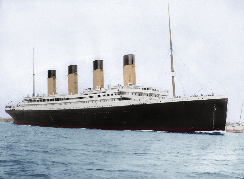
theme_titanic(): the Vallejo Titanic Colors paint set (black, yellow, canvas, anti-fouling red, faded yellow, stone, and wood deck) with a Libre Caslon Display title. Below we simulate how many times teens and adults saw the movie.
set.seed(1997)
fans <- data.frame(age_group = sample(c("Teen", "Adult"), 300, replace = TRUE),
  viewings = sample(c("Once", "Twice", "3+ times"), 300, replace = TRUE))
ggplot(fans, aes(x = age_group, fill = viewings)) +
  geom_bar(position = "fill") +
  labs(title = "Titanic (simulated)", x = NULL, y = "Share", fill = "Viewings") +
  theme_titanic(base_size = 13)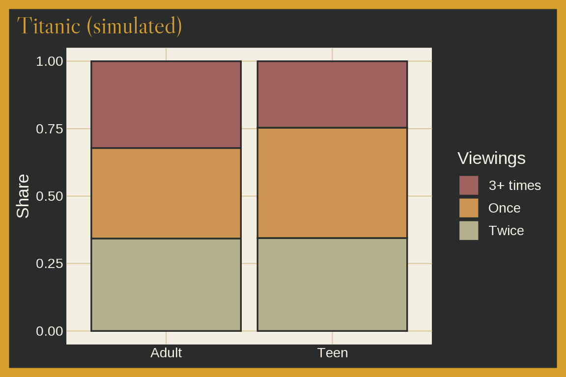
Two-way pagers
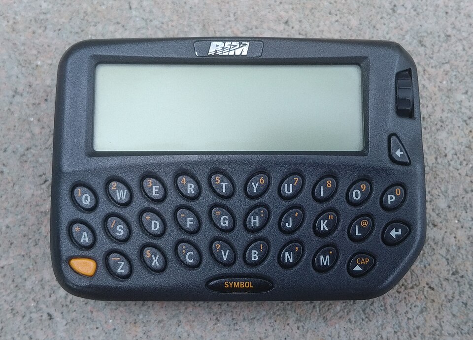
theme_pager() uses a RIM 950 pager on concrete: a charcoal frame and title, a pale LCD panel, charcoal, orange, and slate marks, and an Archivo Black title. Below we simulate the messages one pager received in each hour of a workday.
set.seed(1998)
pages <- data.frame(hour = 7:20)
pages$messages <- rpois(nrow(pages), 2 + 10 * dnorm(pages$hour, 13, 3) / dnorm(0, 0, 3))
ggplot(pages, aes(x = hour, y = messages)) +
  geom_col() +
  labs(title = "Messages by hour", caption = "Simulated data", x = "Hour", y = "Messages") +
  theme_pager(base_size = 13)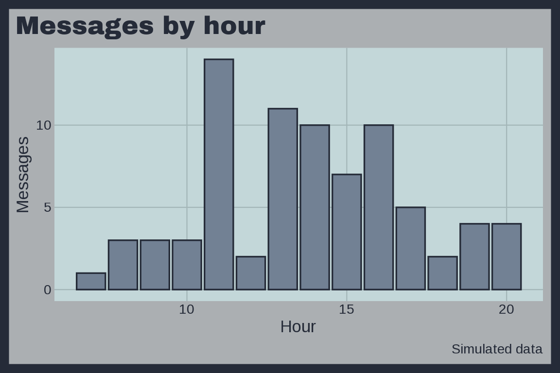
VRML
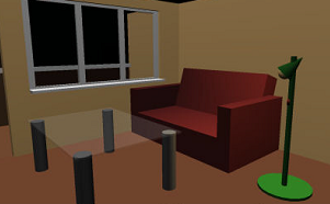
theme_vrml() uses a VRML living room: a tan wall background, a floor brown frame, a pale panel, sofa red, lamp green, black, and glass marks, and an Fira Mono title. Below we simulate render times for four VRML scenes.
set.seed(1996)
scenes <- data.frame(scene = rep(c("Living room", "Garden", "Office", "Museum"), each = 40),
  polygons = round(runif(160, 500, 20000)))
scenes$seconds <- 0.5 + scenes$polygons / 4000 + rnorm(160, 0, 0.4)
ggplot(scenes, aes(x = polygons, y = seconds, color = scene)) +
  geom_point() +
  labs(title = "VRML render times", caption = "Simulated data", x = "Polygons", y = "Seconds to render", color = NULL) +
  theme_vrml(base_size = 13)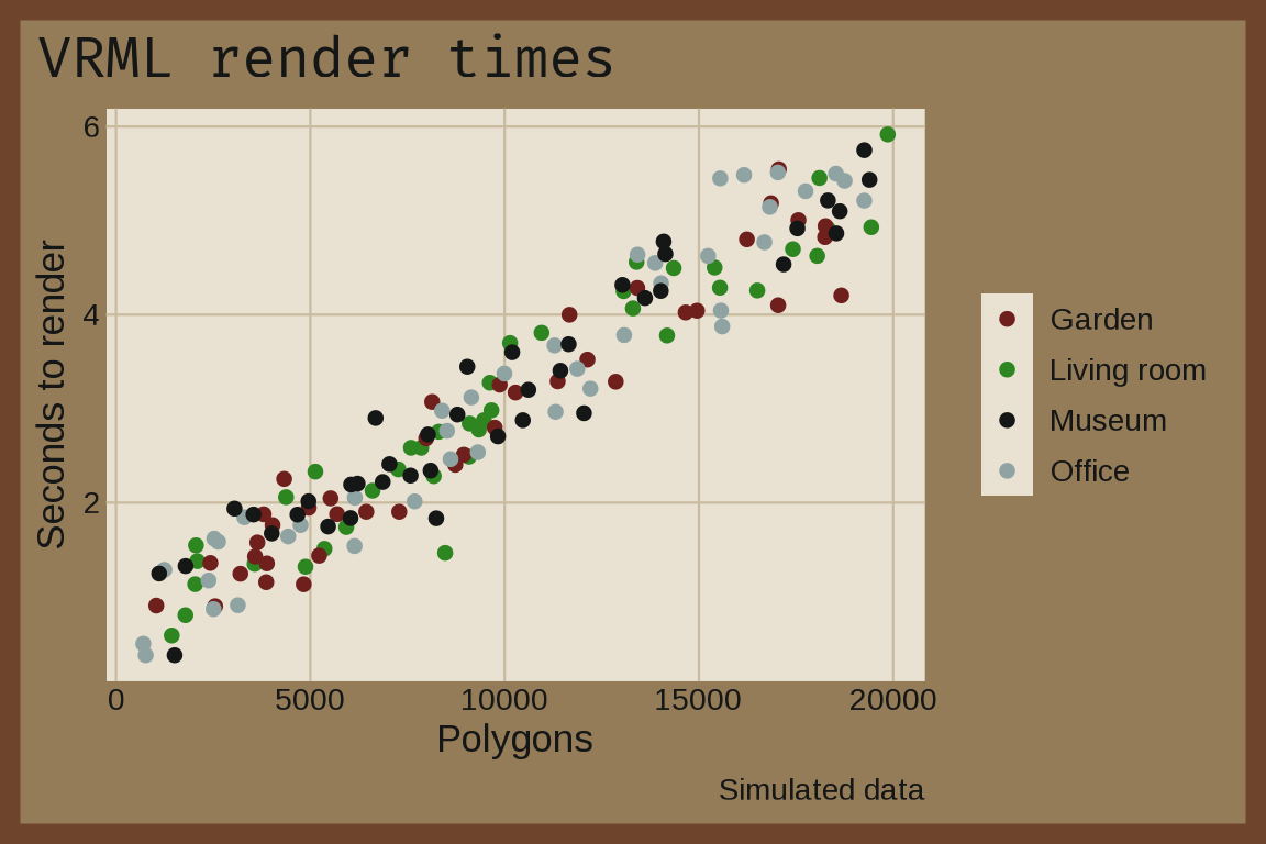
WIRED
theme_wired() uses the WIRED (US) November/December 2024 “Big Interview” cover: a black background, a white frame, a bold Arimo title, and the cover’s red, blue, pink, gray, and steel blue marks. Below we simulate the lengths of 400 interviews in two formats.

set.seed(2024)
qa <- runif(400) < 0.6
interviews <- data.frame(format = ifelse(qa, "Q&A", "Profile"),
  minutes = round(ifelse(qa, rnorm(400, 45, 10), rnorm(400, 90, 20))))
ggplot(interviews, aes(x = minutes, fill = format)) +
  geom_density(alpha = 2/3) +
  labs(title = "WIRED interviews", caption = "Simulated data",
       x = "Interview length (minutes)", fill = NULL) +
  theme_wired(base_size = 13)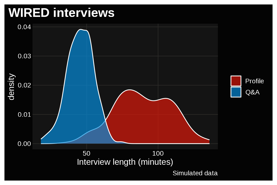
With mode = "light":
last_plot() + theme_wired(base_size = 13, mode = "light")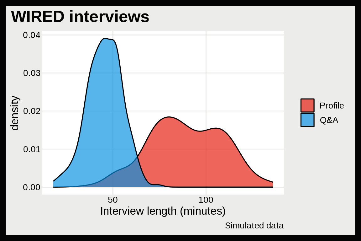
Y2K
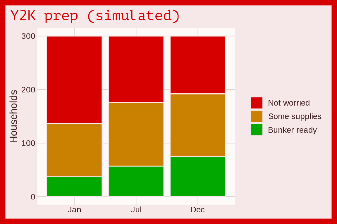
theme_y2k(): LED red, terminal amber and green on black. Below we show how 300 households prepared for Y2K across three surveys.
prep <- data.frame(
  survey = factor(rep(c("Jan", "Jul", "Dec"), each = 3), levels = c("Jan", "Jul", "Dec")),
  level = factor(rep(c("Not worried", "Some supplies", "Bunker ready"), 3),
                 levels = c("Not worried", "Some supplies", "Bunker ready")),
  households = c(163, 100, 37, 124, 119, 57, 108, 117, 75))
ggplot(prep, aes(x = survey, y = households, fill = level)) +
  geom_col() +
  labs(title = "Y2K prep (simulated)", x = NULL, y = "Households", fill = NULL) +
  theme_y2k(base_size = 13)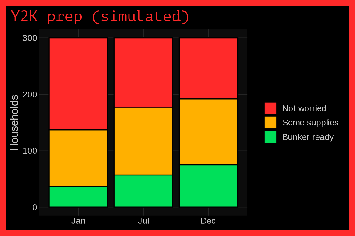
With mode = "light":


Fonts
theme_gameboy() and theme_tetris() use Press Start 2P, which ships with ggrewindr. The other themes use open source fonts from Google Fonts, and they ship with ggrewindr too. Each font keeps its license (SIL Open Font License or Apache License) next to it in the assets folder (see font_path()), so the themes look the same on macOS, Windows, and Linux.
These themes use Arimo for the body text and a display font for the title:
- Anton (
theme_blockbuster()) - Archivo Black (
theme_n64()andtheme_freshprince()) - Macondo (
theme_jurassic()) - Varela Round (
theme_happymeal()) - Caveat (
theme_pogs()) - Barlow Condensed (
theme_walkman()) - Cousine (
theme_oksoda()) - Kaushan Script (
theme_talkboy()) - Arimo (
theme_wired()) - Permanent Marker (
theme_orbitz()) - Tinos (
theme_netscape()) - Libre Caslon Display (
theme_titanic()) - Varela Round (
theme_koosh()) - Jost (
theme_tamagotchi()) - Archivo Black (
theme_supersoaker()) - Uncial Antiqua (
theme_goosebumps()) - Marcellus (
theme_squeezit()) - Fira Mono (
theme_oregontrail()) - Varela Round (
theme_aim()) - Archivo Narrow (
theme_rzone()) - Barlow Condensed (
theme_batman()) - Archivo Black (
theme_snick()) - Yellowtail (
theme_savedbythebell()) - Cabin (
theme_hypercolor()) - PT Mono (
theme_y2k()) - Patrick Hand (
theme_gushers()) - Anton (
theme_doom()) - Russo One (
theme_consolewars()) - Special Elite (
theme_seinfeld()) - Cormorant SC (
theme_powerrangers()) - Arvo (
theme_bopit()) - Comic Neue (
theme_geocities()) - Barlow (
theme_surge()) - Tinos (
theme_microdrive()) - Cabin (
theme_netware()) - Archivo Narrow (
theme_j2me()) - Jost (
theme_palmpilot()) - Fira Sans (
theme_visor()) - Archivo Black (
theme_pager()) - Noto Sans (
theme_cuseeme()) - Fira Mono (
theme_vrml()) - Noto Sans (
theme_javaapplet()) - Permanent Marker (
theme_cuecat()) - Varela Round (
theme_audrey())
When a font file can’t be found, the theme falls back to "sans". You can also pass any family you’ve registered with sysfonts::font_add():
theme_oksoda(base_family = "sans", title_family = "sans")Using a theme for a whole document
Set a theme once in the setup chunk with theme_set(), and the plotting code after it doesn’t need a theme_*() call.
ggplot2::theme_set(ggrewindr::theme_oksoda(base_size = 15))The same works for the light version of a dark theme:
ggplot2::theme_set(ggrewindr::theme_doom(base_size = 15, mode = "light"))