library(dplyr)
library(readr)
library(ggplot2)
library(forcats)

recessions <- read_csv("data/recessions_clean.csv") |>
  mutate(generation_label = fct_reorder(generation_label, entry_start))

era_colors <- c(
  "Dot-com bust" = "#d62728", "Financial crisis" = "#1f77b4",
  "COVID-19" = "#2ca02c", "Other" = "grey50"
)

gen_colors <- c(
  "Greatest Generation" = "#E69F00", "Silent Generation" = "#56B4E9",
  "Baby Boomers" = "#009E73", "Generation X" = "#CC79A7",
  "Millennials" = "#0072B2", "Generation Z" = "#D55E00"
)Recessions
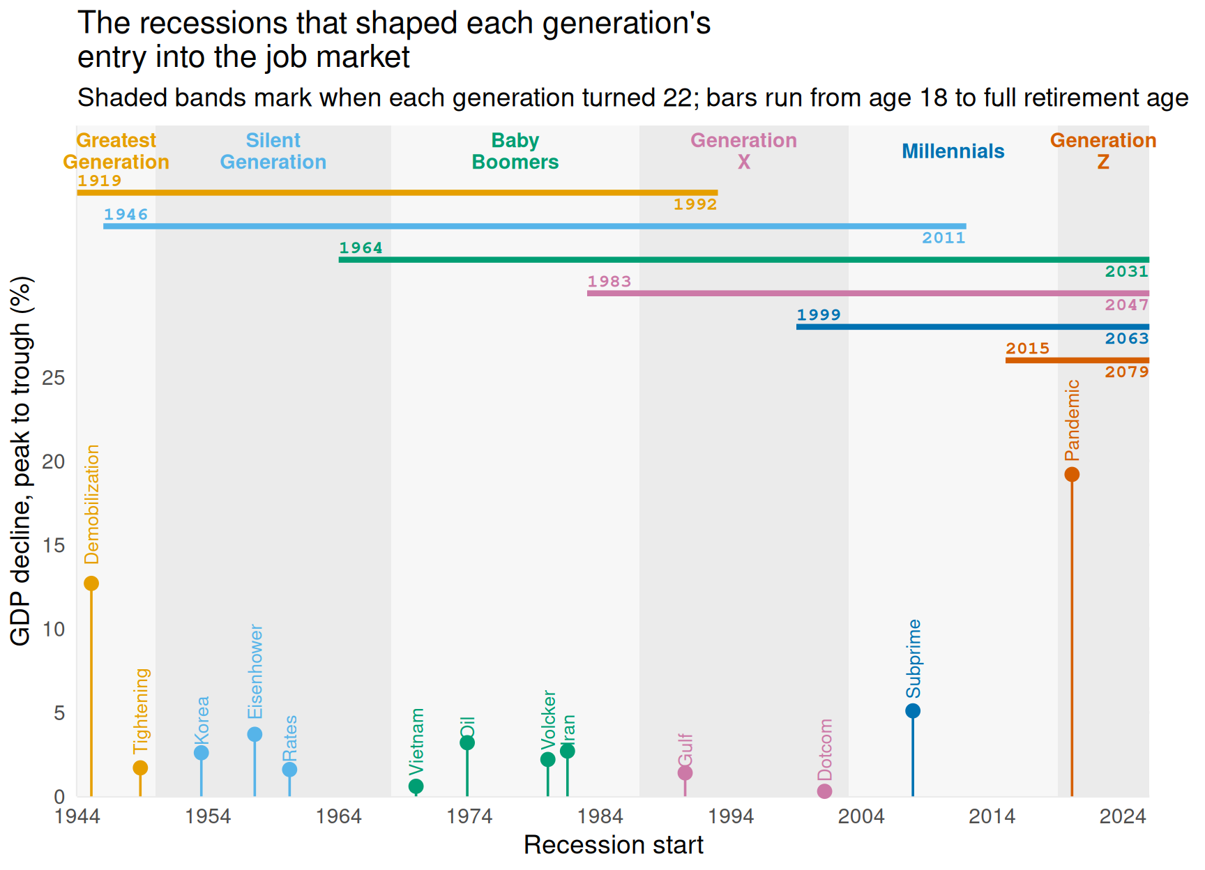
This page plots the recessions that shaped when each generation entered the job market. A generation “experienced” a recession if the recession overlapped the years that generation turned 22, the typical career-entry age. The code below reads the data cleaned in clean_recessions.qmd and plots it two ways.
Timeline
Each lollipop marks a recession’s start date and GDP decline. The shaded bands are each generation’s entry window (age 22), so each recession sits inside the band of the generation it hit. The bars across the top run from when each generation’s oldest members turned 18 to when its youngest members reach full retirement age, labeled with both years. Bars that run past 2025 stop at the edge of the chart. Each generation has its own color, shared by its band label, its bar, and the recessions it experienced.
generations <- distinct(
  recessions, generation, band_start, band_end, band_mid, band_label, shade,
  workforce_start, retirement_year, bar_start, bar_end
) |>
  mutate(bar_y = 26 + 2 * (n() - rank(workforce_start)))

ggplot(recessions) +
  geom_rect(
    data = generations,
    aes(xmin = band_start, xmax = band_end, ymin = -Inf, ymax = Inf, fill = shade),
    show.legend = FALSE
  ) +
  geom_text(
    data = generations,
    aes(x = band_mid, y = 38.5, label = band_label, color = generation),
    size = 3.8, fontface = "bold", lineheight = 0.9
  ) +
  geom_segment(
    data = generations,
    aes(
      x = bar_start, xend = bar_end, y = bar_y, yend = bar_y,
      color = generation
    ),
    linewidth = 1.5
  ) +
  geom_text(
    data = generations,
    aes(x = bar_start, y = bar_y + 0.7, label = workforce_start, color = generation),
    hjust = 0, size = 3.5, fontface = "bold", family = "mono"
  ) +
  geom_text(
    data = generations,
    aes(x = bar_end, y = bar_y - 0.7, label = retirement_year, color = generation),
    hjust = 1, size = 3.5, fontface = "bold", family = "mono"
  ) +
  geom_segment(aes(x = start_date, xend = start_date, y = 0, yend = gdp_decline_pct, color = generation)) +
  geom_point(aes(x = start_date, y = gdp_decline_pct, color = generation), size = 3) +
  geom_text(
    aes(x = start_date, y = gdp_decline_pct, label = name, color = generation),
    angle = 90, hjust = -0.15, size = 3.5
  ) +
  scale_fill_manual(values = c("TRUE" = "grey92", "FALSE" = "grey97")) +
  scale_color_manual(values = gen_colors) +
  scale_x_date(date_breaks = "10 years", date_labels = "%Y", expand = c(0, 0)) +
  scale_y_continuous(limits = c(0, 40), breaks = seq(0, 25, 5), expand = c(0, 0)) +
  coord_cartesian(clip = "off") +
  labs(
    x = "Recession start", y = "GDP decline, peak to trough (%)",
    title = "The recessions that shaped each generation's\nentry into the job market",
    subtitle = "Shaded bands mark when each generation turned 22; bars run from age 18 to full retirement age"
  ) +
  theme_minimal(base_size = 14) +
  theme(
    panel.grid.minor = element_blank(), legend.position = "none",
    plot.margin = margin(5.5, 30, 5.5, 5.5)
  )
By generation
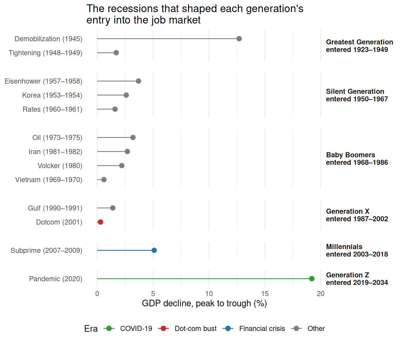
The chart below groups the same recessions by generation. Each row’s height is proportional to the number of recessions that generation faced as it entered the job market.
ggplot(recessions, aes(x = gdp_decline_pct, y = fct_reorder(label, gdp_decline_pct), color = era)) +
  geom_segment(aes(x = 0, xend = gdp_decline_pct, yend = fct_reorder(label, gdp_decline_pct))) +
  geom_point(size = 2.5) +
  facet_grid(generation_label ~ ., scales = "free_y", space = "free_y") +
  scale_color_manual(values = era_colors) +
  labs(
    x = "GDP decline, peak to trough (%)", y = NULL, color = "Era",
    title = "The recessions that shaped each generation's\nentry into the job market"
  ) +
  theme_minimal() +
  theme(
    strip.text.y = element_text(face = "bold", angle = 0, hjust = 0),
    panel.grid.major.y = element_blank(),
    panel.spacing.y = unit(1, "lines"),
    legend.position = "bottom"
  )