bad_80 = portfolio_return(stock_pct=0.80, stock_return=-0.40, bond_return=0.0)
avg_80 = portfolio_return(stock_pct=0.80, stock_return=0.10, bond_return=0.04)
bad_80, avg_80
(-0.32000000000000006, 0.08800000000000001)Your asset allocation is how you split your investments between stocks and bonds. It does more to decide how your money grows (and how bumpy the ride feels) than which funds you pick. Asset allocation math answers two questions. What does a split do in a good year and a bad year? And how much do you move when you rebalance? In this page I’ll answer both with portfolio_return() and rebalance_amount(), using the numbers from the Asset Allocation chapter of the book.
Both functions accept arrays and follow the conventions in Get started: shares and returns are decimals. portfolio_return() also accepts polars expressions, so it works inside with_columns().
| Function | Returns | Units |
|---|---|---|
| portfolio_return() | the return on a stock and bond split | decimal (-0.32 is a 32% loss) |
| rebalance_amount() | how much to buy or sell to reach a target | dollars (positive buys, negative sells) |
The chapter splits $10,000 three ways: 100/0, 80/20, and 60/40 (stocks/bonds). It assumes stocks earn 10% in an average year and lose 40% in a bad year. Bonds earn 4% in an average year and break even in a bad year. These are round numbers for illustration, not predictions.
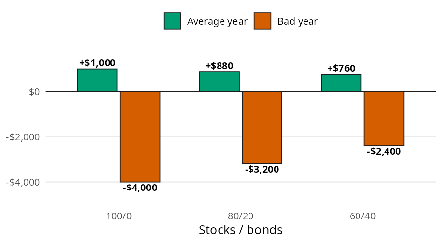
Each bar is a weighted average: the stock return times the share in stocks, plus the bond return times the share in bonds. portfolio_return() takes the share in stocks and the two returns. Here is the 80/20 split in a bad year and an average year:
bad_80 = portfolio_return(stock_pct=0.80, stock_return=-0.40, bond_return=0.0)
avg_80 = portfolio_return(stock_pct=0.80, stock_return=0.10, bond_return=0.04)
bad_80, avg_80(-0.32000000000000006, 0.08800000000000001)In a bad year the 80/20 split loses 32%, or $3,200 on $10,000. In an average year it gains 8.8%, or $880. The result is a decimal, so multiply by the balance to get dollars.
Your split won’t stay where you set it. The chapter starts with $10,000 at 80/20 ($8,000 in stocks and $2,000 in bonds), then stocks drop 30%. The stock part of the bar shrinks to $5,600, the total falls to $7,600, and stocks are now only about 74% of it.
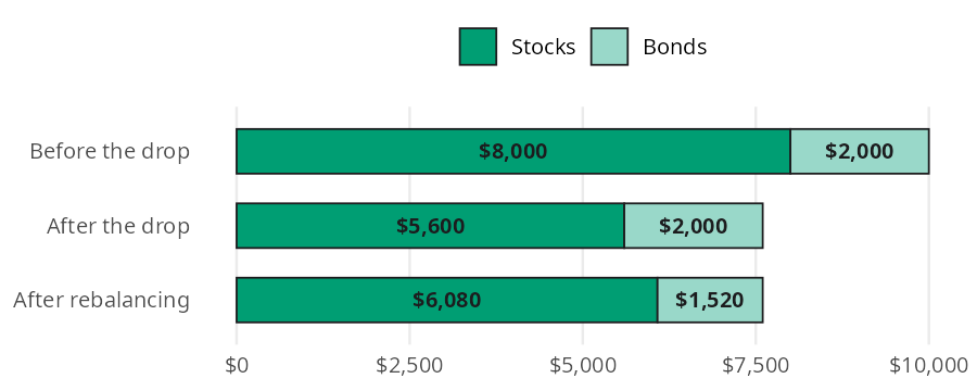
Rebalancing moves just enough from bonds to stocks to get back to 80/20. The target for stocks is 80% of the new total, and rebalance_amount() returns the difference between that target and what you hold:
move = rebalance_amount(target_pct=0.80, total=5600 + 2000, current_amount=5600)
move480.0A positive answer means buy. You move $480 from bonds into stocks, which means buying stocks while they’re down. That’s exactly what rebalancing is for.
The chapter’s Python code builds all three splits at once with polars. Because portfolio_return() accepts pl.col("stocks"), it works inside with_columns() like any other expression. Multiplying by the $10,000 balance gives the dollar labels from the bar model:
pl.DataFrame({"stocks": [1.0, 0.8, 0.6]}).with_columns(
    average=portfolio_return(pl.col("stocks"), 0.10, 0.04),
    bad=portfolio_return(pl.col("stocks"), -0.40, 0.0),
).with_columns(
    average_dollars=pl.col("average") * 10000,
    bad_dollars=pl.col("bad") * 10000,
)| stocks | average | bad | average_dollars | bad_dollars |
|---|---|---|---|---|
| f64 | f64 | f64 | f64 | f64 |
| 1.0 | 0.1 | -0.4 | 1000.0 | -4000.0 |
| 0.8 | 0.088 | -0.32 | 880.0 | -3200.0 |
| 0.6 | 0.076 | -0.24 | 760.0 | -2400.0 |
Moving from 100/0 to 60/40 gives up $240 in an average year and saves $1,600 in a bad one.
rebalance_amount() takes arrays, so one call rebalances every fund in a portfolio. Suppose the chapter’s three fund portfolio (60% US stocks, 30% international stocks, 10% bonds) has drifted to $6,600, $2,500, and $900:
current = [6600, 2500, 900]
pl.DataFrame({
    "fund": ["US stocks", "international stocks", "bonds"],
    "target_pct": [0.60, 0.30, 0.10],
    "current": current,
    "move": rebalance_amount(
        target_pct=[0.60, 0.30, 0.10], total=sum(current), current_amount=current
    ),
})| fund | target_pct | current | move |
|---|---|---|---|
| str | f64 | i64 | f64 |
| "US stocks" | 0.6 | 6600 | -600.0 |
| "international stocks" | 0.3 | 2500 | 500.0 |
| "bonds" | 0.1 | 900 | 100.0 |
Sell $600 of US stocks and use it to buy the other two. The moves add up to zero, because rebalancing only shifts money between funds.
Both functions are simple on purpose:
total has to include current_amount.Here is the chapter’s bad year from start to finish. $10,000 at 80/20 meets a 30% stock drop, and bonds break even. portfolio_return() gives the loss on the whole portfolio, and rebalance_amount() gives the move:
drop = portfolio_return(stock_pct=0.80, stock_return=-0.30, bond_return=0.0)
after_drop = 10000 * (1 + drop)
to_stocks = rebalance_amount(
    target_pct=0.80, total=after_drop, current_amount=8000 * (1 - 0.30)
)
drop, after_drop, to_stocks
(-0.24, 7600.0, 480.0)The portfolio falls 24% to $7,600, and rebalancing moves $480 into stocks. How long until it’s back to $10,000? If the next years are average ones, the 80/20 split grows at 8.8% a year, and future_value() from Investing Basics shows the path:
recovery_years = [1, 2, 3, 4]
pl.DataFrame({
    "years": recovery_years,
    "value": future_value(present_value=after_drop, rate=avg_80, years=recovery_years),
})| years | value |
|---|---|
| i64 | f64 |
| 1 | 8268.8 |
| 2 | 8996.4544 |
| 3 | 9788.142387 |
| 4 | 10649.498917 |
The portfolio is back above $10,000 in year 4. Staying invested (and rebalancing into the drop) is what makes the recovery possible.
Asset allocation is how you split your money between stocks and bonds, and it matters more than which funds you pick. portfolio_return() shows what a split does in a good year and a bad one, and it works on polars columns as well as numbers. rebalance_amount() shows how much to move to get back on target, which makes you buy low without predicting anything.