5 Documentation

Published

2026-10-15

In the Development Workflow chapter, we settled into a loop of editing code in src/pyap/, saving, and checking the result. pyap installs and runs, but the only documentation was a single sentence on scatter_plot() and another in __init__.py. This means anyone opening the package (including me, six months from now) would need to read the function body to learn what each argument expects and what comes back.

This chapter fixes that by writing complete docstrings for the code in pyap, then rendering them into an HTML documentation site.

Comparison to R package documentation

If you’ve read the Documentation chapter of Shiny App-Packages, you’ll know we document app-package functions with roxygen2:

Help documentation is created by placing #' comments above each function
Tags like @title and @description are used to organize the documentation
We run devtools::document() to turn them into .Rd files in man/

Python stores docstrings on the function itself, so help() can read it the moment the module is imported. I’ve found this shifts the work from running tools to writing well, so most of this chapter is about what goes inside the triple quotes.

5.1 Diverging branches

Chapters 1 to 4 built pyap in a straight line: each branch started where the previous one ended. Going forward, some of the branches will diverge. I’ve done this to try and accurately demonstrate how Python package development goes. In R, documentation is limited to roxygen2 tags (and pkgdown for building package websites). But as with most things in Python, there are several valid tools for the same job.

For example, from what I’ve seen, there are at least two excellent ways to turn docstrings into package documentation with a website (and a third, great-docs, which we’ll cover in a later chapter). So, in this chapter, I’d rather show a working version of each option than pretend there’s only one. The branches in this chapter are here to illustrate alternatives (different tools for the same step).

The diagram below shows the branches in this chapter:

%%{init: {'theme': 'neutral', 'themeVariables': { 'fontFamily': 'monospace', "fontSize":"14px"}}}%%

flowchart LR
    B4["<strong>04_dev</strong><br/>edit, sync,<br/>run loop"]
    B51["<strong>05.1_pdoc</strong><br/>docstrings +<br/><code>pdoc</code>"]
    B6["<strong>06_dependencies</strong><br/>next chapter"]
    B52["<strong>05.2_mkdocs</strong><br/><code>mkdocs</code> +<br/><code>mkdocstrings</code>"]

    B4 --> B51 --> B6
    B51 -.->|"alternative"| B52

    classDef project fill:#553c9a,stroke:#b794f4,color:#fff
    classDef uvStyle fill:#744210,stroke:#f6ad55,color:#fff
    classDef pkg fill:#2d3748,stroke:#48bb78,color:#fff

    class B4 project
    class B51,B6 pkg
    class B52 uvStyle

The main line and a side branch

05.1_pdoc adds the docstrings and builds the documentation with pdoc. 05.2_mkdocs starts from 05.1_pdoc, keeps the docstrings, and swaps pdoc for mkdocs. The dotted arrow marks it as a side branch: the Dependencies chapter will build on 05.1_pdoc.

Let’s dive into docstrings!

5.2 What is a docstring?

A docstring is a string literal placed as the first statement in a module, function, or class. Python doesn’t discard it like a comment. It attaches the string to the object as its __doc__ attribute, which is what makes docstrings readable from the console, the editor, and documentation tools.

Comparison to R package documentation

A string literal is a string value written directly in the code, between quotes ("movies.csv" or 'IMDB rating'), rather than one built by an expression or stored in a variable. R has string literals too ("movies.csv", and raw strings like r"(C:\path)" since R 4.0), but R doesn’t treat a string at the top of a function body as documentation.

If we placed "Create a scatter plot" as the first line of an R function, R would evaluate it, discard the result, and move on. This is why R documentation lives outside the function code, in roxygen2 comments that document() turns into .Rd files.

By convention, docstrings are written inside three consecutive double quotes: """docstring text""". In the 04_dev branch, if we open src/pyap/utils.py, we can see a docstring for scatter_plot():

def scatter_plot(df, x_var, y_var, col_var, alpha_var, size_var, title=""):
    """Create a scatter plot of df colored by a categorical variable."""

A comment in the same position (# Create a scatter plot...) would look almost identical in the editor, but it would be invisible to everything below.

5.2.1 Where Python reads docstrings

The fastest way to read a docstring is help() in a Python console (Positron’s Console, or uv run python from the project root in a terminal). We’ll import the function and pass it to help():

>>> from pyap.utils import scatter_plot
>>> help(scatter_plot)

Help on function scatter_plot in module pyap.utils: scatter_plot(df, x_var, y_var, col_var, alpha_var, size_var, title='') Create a scatter plot of df colored by a categorical variable.

The output above is from a terminal, where help() opens a pager (press q to return to the prompt). In Positron, help() displays the function’s signature and docstring in the Help pane:

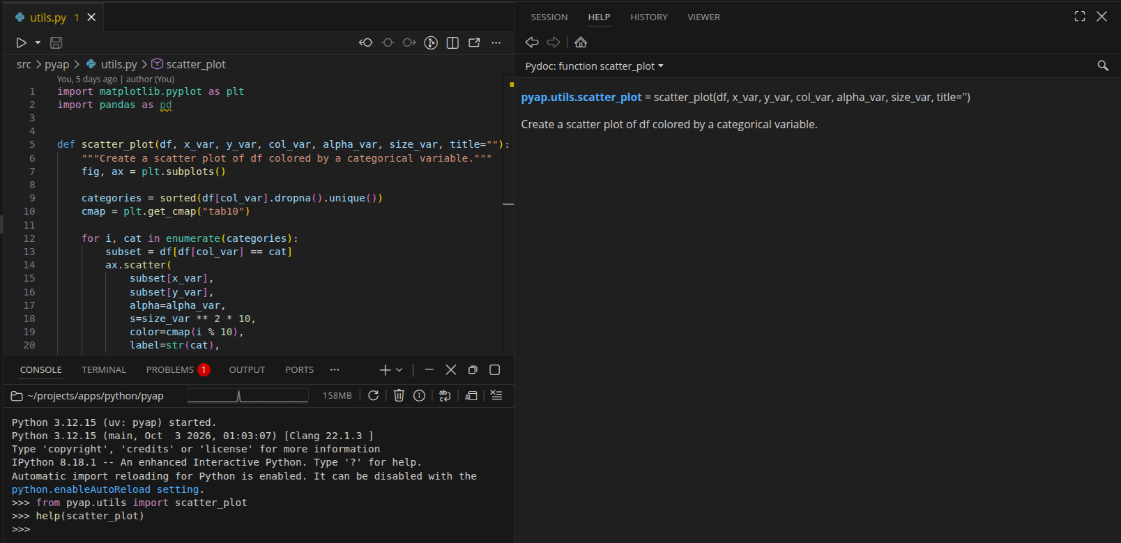
The raw string is available on the __doc__ attribute:

>>> scatter_plot.__doc__

'Create a scatter plot of df colored by a categorical variable.'

Modules and packages have docstrings too. pyap.__doc__ returns the sentence in src/pyap/__init__.py from the Python Packages chapter, and help(pyap) shows the package docstring along with its contents. In a terminal, the contents list both app and utils, but Positron’s Help pane only listed utils (the module we had already imported):

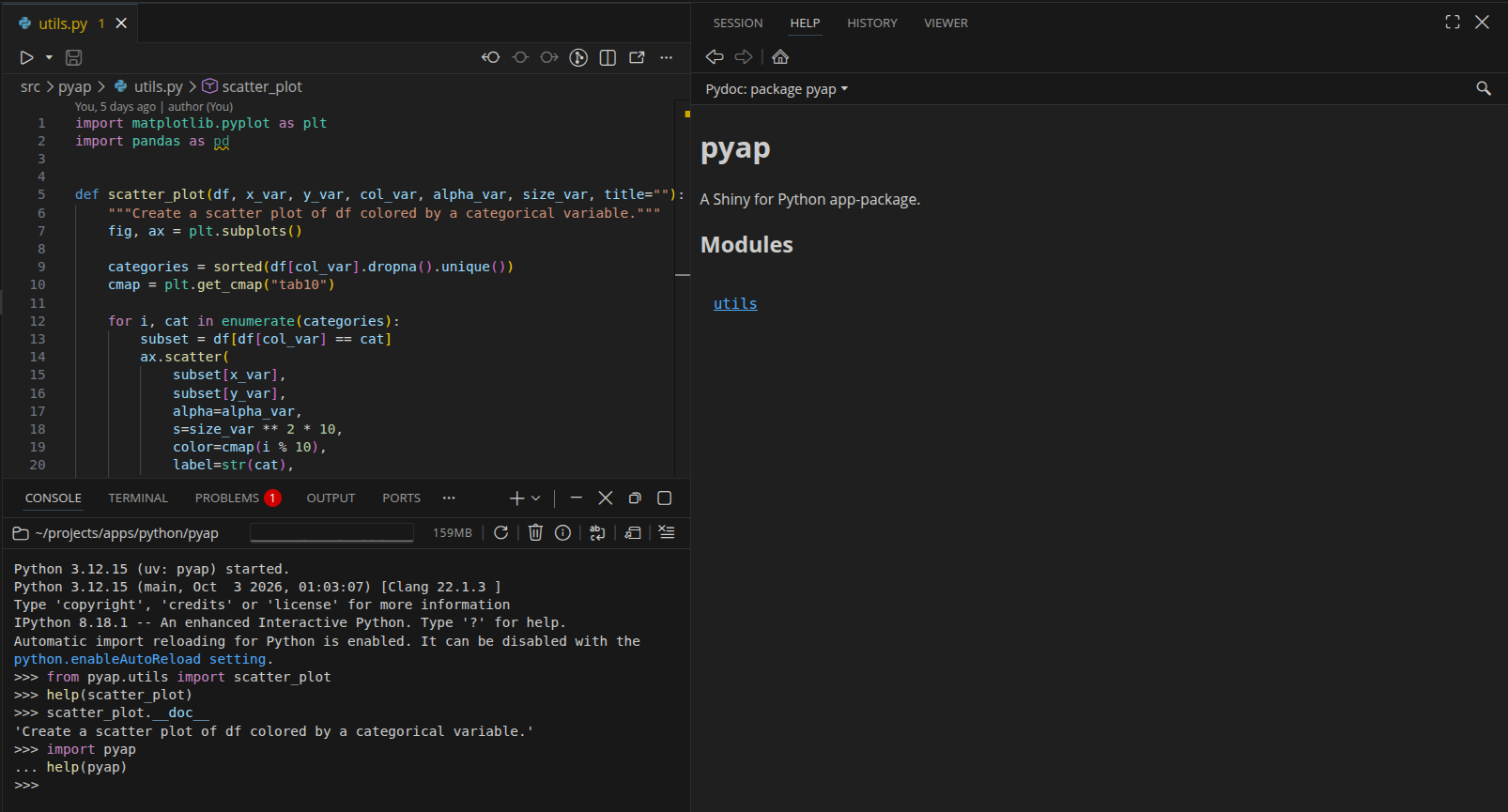
Editors read docstrings as well. In Positron, hovering over scatter_plot in app.py shows its signature and docstring in a tooltip, and the same text appears in the signature help while we type the arguments.

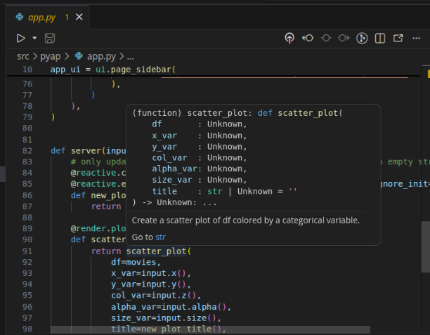
The diagram below shows the two routes a docstring takes from our source files to a reader:

%%{init: {'theme': 'neutral', 'themeVariables': { 'fontFamily': 'monospace', "fontSize":"14px"}}}%%

flowchart LR
    Src(["docstrings in<br/><code>src/pyap/*.py</code>"])

    subgraph Runtime["<strong>Imported</strong>"]
        Doc("<code>__doc__</code><br/>on each object")
        Help("<code>help()</code><br/>in the console")
        Pdoc("<code>pdoc</code>")
    end

    subgraph Static["<strong>Read from source</strong>"]
        Hover("editor hover<br/>(Positron)")
        Mk("<code>mkdocstrings</code>")
    end

    Site[\"HTML<br/>documentation site"\]

    Src -->|"import"| Doc
    Doc --> Help
    Doc --> Pdoc
    Src -->|"parse"| Hover
    Src -->|"parse"| Mk
    Pdoc --> Site
    Mk --> Site

    classDef srcStyle fill:#2d3748,stroke:#48bb78,color:#fff
    classDef runStyle fill:#744210,stroke:#f6ad55,color:#fff
    classDef staticStyle fill:#553c9a,stroke:#b794f4,color:#fff
    classDef siteStyle fill:#2c5282,stroke:#63b3ed,color:#fff

    class Src srcStyle
    class Doc,Help,Pdoc runStyle
    class Hover,Mk staticStyle
    class Site siteStyle

Where docstrings are read

Docstrings live in the source files, and they reach readers by two routes:

The top route imports pyap and reads __doc__ from the live objects. help() works this way, and so does pdoc, which we’ll use to build the HTML site.
The bottom route parses the .py files without running them. Editors typically use a language server for hover text, and mkdocstrings (a plugin for mkdocs) reads source files by default.

The difference matters for pyap, because importing pyap.app runs code (we’ll come back to this when we build the site). Every route reads the same string. There’s no generated help folder to keep in sync, so the docstring in the source file is the documentation.

5.3 Writing docstrings

The docstrings in this section (and the pdoc site in the next one) are on the 05.1_pdoc branch. Check it out to follow along, and sync the environment:

git checkout 05.1_pdoc

uv sync

The branch adds docstrings to all three modules in src/pyap/, adds pdoc to the dev dependency group (pyproject.toml and uv.lock), and adds docs/ to .gitignore. The project structure is below:

pyap/ ├── .gitignore ├── .python-version ├── .vscode/ │ └── settings.json ├── README.md ├── movies.csv ├── pyproject.toml ├── src/ │ └── pyap/ │ ├── __init__.py │ ├── app.py │ └── utils.py └── uv.lock

Unlike roxygen2, which generates .Rd files in man/, docstrings add no files to the package. Documentation in Python lives inside the files we already have, which is why the tree looks exactly like the one from the 04_dev branch.

5.3.1 PEP 257 basics

PEP 257 sets the ground rules every docstring convention builds on. The ones we’ll follow in pyap are:

Use triple double quotes ("""), even for one line docstrings.
Start with a one line summary that fits on the first line and ends with a period. PEP 257 recommends the imperative mood (“Create a scatter plot”, not “Creates a scatter plot”).
For longer docstrings, leave a blank line after the summary, then add the details. Put the closing """ on a line by itself.
Place the docstring as the first statement in the body (or at the top of the file, for a module docstring).

The existing docstring on scatter_plot() in src/pyap/utils.py already follows the first two rules. The summary line deserves extra attention, because it’s the line tools show in package indexes and tooltips. PEP 257 doesn’t say anything about how to describe arguments or return values, though. That job belongs to a docstring convention (which we’ll cover below).

5.3.2 Choosing a convention

A docstring convention is just an agreed set of section headings and layouts, so people and tools know where to find the parameters, the return value, and the examples.¹ The two most common conventions in data science code are described below:

NumPy style: section titles underlined with dashes, and each parameter on its own line followed by its type.
Google style: section titles followed by a colon (Args:, Returns:), with each parameter indented beneath.

The Whole Game chapter used Google style for geyser_waiting(), and it’s a fine choice. For the remaining branches in pyap, I’ll switch to NumPy style because pandas, numpy, and matplotlib (all three of the packages scatter_plot() depends on) document their functions this way, so our help pages will read like the ones I consulted while writing the code. NumPy style also has more room for longer descriptions, which helps when an argument needs a sentence or two of explanation.

The convention matters less than consistency. Pick one convention for the entire package, and tell the documentation tools which one you picked (we’ll do this with a flag below).

5.3.3 Function docstrings

A NumPy style function docstring has a summary line, an extended description, and a series of sections. The summary line and description for scatter_plot() are below:

show/hide summary and description

def scatter_plot(df, x_var, y_var, col_var, alpha_var, size_var, title=""):
    """Create a scatter plot colored by a categorical variable.

    Draws one scatter layer per category in `col_var`, so each category
    gets its own color and legend entry. Axis labels and the legend title
    are built from the column names (underscores become spaces, and each
    word is capitalized).
    """

The summary line plays the role of @title, and the extended description plays the role of @description.

Each section below is part of the same docstring, and maps to something a reader would otherwise have to work out from the code:

`Parameters`

Parameters need one entry per argument, written as name : type with the description indented below it. Optional arguments add optional after the type.

show/hide Parameters section

def scatter_plot(df, x_var, y_var, col_var, alpha_var, size_var, title=""):
    """
    Parameters
    ----------
    df : pandas.DataFrame
        Data containing the columns named in `x_var`, `y_var`, and
        `col_var`.
    x_var : str
        Name of the numeric column mapped to the x axis.
    y_var : str
        Name of the numeric column mapped to the y axis.
    col_var : str
        Name of the categorical column used to color the points. Rows
        with a missing value in this column are not plotted.
    alpha_var : float
        Point transparency, from 0 (transparent) to 1 (opaque).
    size_var : float
        Point size. The marker area is `size_var ** 2 * 10`.
    title : str, optional
        Plot title. The default (an empty string) leaves the plot
        untitled.
    """

`Returns`

The Returns section should include the type of the returned object and a short description. scatter_plot() returns the figure rather than drawing it, which is what @render.plot expects.

show/hide Returns section

def scatter_plot(df, x_var, y_var, col_var, alpha_var, size_var, title=""):
    """
    Returns
    -------
    matplotlib.figure.Figure
        The figure holding the scatter plot.
    """

`Notes`

Notes can be any details that don’t belong to a single argument. The tab10 limit is easy to miss until a column has more than ten categories.

show/hide Notes section

def scatter_plot(df, x_var, y_var, col_var, alpha_var, size_var, title=""):
    """
    Notes
    -----
    Colors come from the matplotlib `tab10` colormap, which repeats
    after ten categories.
    """

`Examples`

Like @examples in roxygen2, the Examples section holds code a reader can paste into the console, written in the >>> prompt format.²

show/hide Examples section

def scatter_plot(df, x_var, y_var, col_var, alpha_var, size_var, title=""):
    """
    Examples
    --------
    >>> import pandas as pd
    >>> from pyap.utils import scatter_plot
    >>> movies = pd.read_csv("movies.csv")
    >>> fig = scatter_plot(movies, "critics_score", "audience_score",
    ...                    "mpaa_rating", 0.4, 3)
    """

I’ve written the descriptions from the reader’s side of the function. col_var doesn’t just say “column for color”; it also says what happens to missing values, because that’s the question someone debugging a sparse plot will have. This is the same advice I gave for @param in the R book: include the type and what the argument does.

The full docstring for scatter_plot() is below:

show/hide full scatter_plot() docstring

# in src/pyap/utils.py
def scatter_plot(df, x_var, y_var, col_var, alpha_var, size_var, title=""):
    """Create a scatter plot colored by a categorical variable.

    Draws one scatter layer per category in `col_var`, so each category
    gets its own color and legend entry. Axis labels and the legend title
    are built from the column names (underscores become spaces, and each
    word is capitalized).

    Parameters
    ----------
    df : pandas.DataFrame
        Data containing the columns named in `x_var`, `y_var`, and
        `col_var`.
    x_var : str
        Name of the numeric column mapped to the x axis.
    y_var : str
        Name of the numeric column mapped to the y axis.
    col_var : str
        Name of the categorical column used to color the points. Rows
        with a missing value in this column are not plotted.
    alpha_var : float
        Point transparency, from 0 (transparent) to 1 (opaque).
    size_var : float
        Point size. The marker area is `size_var ** 2 * 10`.
    title : str, optional
        Plot title. The default (an empty string) leaves the plot
        untitled.

    Returns
    -------
    matplotlib.figure.Figure
        The figure holding the scatter plot.

    Notes
    -----
    Colors come from the matplotlib `tab10` colormap, which repeats
    after ten categories.

    Examples
    --------
    >>> import pandas as pd
    >>> from pyap.utils import scatter_plot
    >>> movies = pd.read_csv("movies.csv")
    >>> fig = scatter_plot(movies, "critics_score", "audience_score",
    ...                    "mpaa_rating", 0.4, 3)
    """
    # function body unchanged

Types in docstrings and type hints

NumPy style puts each parameter’s type in the docstring. Without type hints, editors can’t infer the types either (the Positron tooltip above shows Unknown for every argument). Python also supports type hints in the function signature (def scatter_plot(df: pd.DataFrame, x_var: str, ...)), and many documentation tools display both. We’ll keep the types in the docstring for now, so the signature in utils.py doesn’t change in this chapter.

5.3.4 Module docstrings

A module docstring describes the file as a whole. It must be the first statement in the file, above the imports.

show/hide scatter plot module docstring

"""Plotting utilities for the pyap movies app.

The functions in this module are plain matplotlib code with no Shiny
dependencies, so they can be called from the app, from a test, or from
the Python console.
"""

import matplotlib.pyplot as plt
import pandas as pd

src/pyap/app.py gets a module docstring too. The # Run with: comment can stay on the first line, because comments aren’t statements; the docstring is still the first statement in the file:

show/hide app module docstring

# Run with: uv run shiny run src/pyap/app.py
"""Shiny app for exploring the movies data.

Defines the UI (`app_ui`), the server function (`server()`), and the
`app` object that `shiny run` looks for. The data are read from
`movies.csv` in the working directory when this module is imported.
"""

from shiny import App, ui, render, reactive
import pandas as pd

from pyap.utils import scatter_plot

The last sentence is a deliberate warning, because reading movies.csv at import time is the behavior that will trip up pdoc below, and the docstring is the right place to tell readers about it until the Data chapter changes it.

5.3.4.1 `server` docstring

The server() function also gets a short docstring. Shiny passes it three objects, so the Parameters section names their types and lists the inputs and outputs the function uses:

show/hide server docstring

def server(input, output, session):
    """Server logic for the movies app.

    Parameters
    ----------
    input : shiny.Inputs
        Input values from the sidebar (`x`, `y`, `z`, `alpha`, `size`,
        `plot_title`, and `update_plot_title`).
    output : shiny.Outputs
        Outputs rendered by the app (`scatterplot`).
    session : shiny.Session
        The current user session.
    """

The rest of app.py is unchanged. The functions defined inside server() (new_plot_title() and scatterplot()) are created each time a session starts, so documentation tools don’t see them; the existing comment above new_plot_title() is the right level of documentation for them.

5.3.5 The package docstring

The docstring in src/pyap/__init__.py is the first thing a reader sees in help(pyap) and on the front page of a documentation site. We’ll keep the summary line from the Python Packages chapter and add a short description that points to the modules:

"""A Shiny for Python app-package.

`pyap` packages the movies review app as an installable Python package.
The app (UI, server, and the `app` object) lives in `pyap.app`, and the
plotting code it calls lives in `pyap.utils`.
"""

A package docstring is a good place for orientation, not detail. The function level docstrings carry the specifics, and the package docstring tells the reader where to look for them.³

5.3.6 Confirming the docstrings

Docstrings are part of the source code, so the editable install picks them up without a sync (this is the No action path from the Development Workflow chapter). A console that already imported pyap.utils still holds the old function, though, so we’ll restart it (or start a new one with uv run python) and call help() again:

>>> from pyap.utils import scatter_plot
>>> help(scatter_plot)

Help on function scatter_plot in module pyap.utils: scatter_plot(df, x_var, y_var, col_var, alpha_var, size_var, title='') Create a scatter plot colored by a categorical variable. Draws one scatter layer per category in `col_var`, so each category gets its own color and legend entry. Axis labels and the legend title are built from the column names (underscores become spaces, and each word is capitalized). Parameters ---------- df : pandas.DataFrame Data containing the columns named in `x_var`, `y_var`, and `col_var`. x_var : str Name of the numeric column mapped to the x axis. y_var : str Name of the numeric column mapped to the y axis. col_var : str Name of the categorical column used to color the points. Rows with a missing value in this column are not plotted. alpha_var : float Point transparency, from 0 (transparent) to 1 (opaque). size_var : float Point size. The marker area is `size_var ** 2 * 10`. title : str, optional Plot title. The default (an empty string) leaves the plot untitled. Returns ------- matplotlib.figure.Figure The figure holding the scatter plot. Notes ----- Colors come from the matplotlib `tab10` colormap, which repeats after ten categories. Examples -------- >>> import pandas as pd >>> from pyap.utils import scatter_plot >>> movies = pd.read_csv("movies.csv") >>> fig = scatter_plot(movies, "critics_score", "audience_score", ... "mpaa_rating", 0.4, 3)

The output should show the full NumPy style docstring below the signature. help() prints the sections as plain text; the underlined headings are what documentation tools look for when they turn the docstring into HTML.

5.4 Rendering documentation to HTML

help() and editor tooltips cover anyone who already has pyap installed. A documentation site covers everyone else (and makes the docstrings searchable). We’ll use pdoc on the 05.1_pdoc branch, build the same site with mkdocs on the 05.2_mkdocs branch, and finish with a short look at great-docs.

5.4.1 Adding `pdoc`

pdoc generates API documentation from a package’s docstrings with no configuration file. We only need it while developing pyap, so we’ll add it to the dev dependency group with --dev:

uv add --dev pdoc

Resolved 50 packages in 310ms Building pyap @ file:///path/to/pyap Built pyap @ file:///path/to/pyap Prepared 5 packages in 169ms Uninstalled 1 package in 1ms Installed 6 packages in 12ms + jinja2==3.1.6 + markdown2==2.5.5 + markupsafe==3.0.4 + pdoc==16.0.0 ~ pyap==0.1.0 (from file:///path/to/pyap) + pygments==2.21.0

uv add updates pyproject.toml, uv.lock, and .venv/ in one step. The new table in pyproject.toml is below:

[dependency-groups]
dev = [
    "pdoc>=16.0.0",
]

Installing pyap never installs pdoc, because dependency groups aren’t part of the package metadata (we covered this in the Python Packages chapter).

5.4.2 Previewing the site

pdoc takes the name of the package to document. With uv run, we’re sure it imports the editable install of pyap from .venv/:

uv run pdoc --docformat numpy pyap

pdoc server ready at http://localhost:8080

This starts a local web server and opens the documentation in the browser. The --docformat numpy flag tells pdoc to read the Parameters, Returns, Notes, and Examples sections as NumPy style (without it, the underlined headings render as plain text). The package docstring becomes the landing page, and pyap.app and pyap.utils each get their own page. Press Ctrl + C in the terminal to stop the server.

pdoc only documents public names. Anything that starts with an underscore is skipped, and if a module defines __all__, only the names it lists are included.⁴

pdoc imports pyap

pdoc builds its pages from the imported package (the top route in the diagram above), and importing pyap.app runs pd.read_csv("movies.csv"). The relative path is resolved from the folder we run pdoc in, so pdoc has to be run from the project root, exactly like the app. From any other folder, the import of pyap.app fails with a FileNotFoundError. The Data chapter removes this dependence on the working directory.

5.4.3 Writing a static site

To write the site to files instead of serving it, we pass an output folder with -o:

uv run pdoc --docformat numpy -o docs pyap

pdoc writes one HTML page per module, plus an index page and a search index. The docs/ folder should look like this:

docs/ ├── index.html ├── pyap/ │ ├── app.html │ └── utils.html ├── pyap.html └── search.js

The pages are self contained, so opening docs/index.html in a browser shows the same site as the preview. The 05.1_pdoc branch lists docs/ in .gitignore, because the HTML can always be rebuilt from the docstrings. We’ll publish it in the Deploy section.

5.5 Building the site with `mkdocs`

pdoc is the simplest way to get from docstrings to HTML, but every page it builds comes from a docstring. When a package needs written guides alongside its reference pages, mkdocs is a common next step. mkdocs builds a site from a folder of Markdown files, and the mkdocstrings plugin inserts API documentation from docstrings into those pages.

The two tools can’t share a project as it’s set up on 05.1_pdoc, because they use docs/ for opposite jobs. pdoc -o docs writes generated HTML into docs/, which is why that branch ignores the folder. mkdocs reads its Markdown sources from docs/, so the folder has to be committed. Rather than pointing one tool at a different folder, the 05.2_mkdocs branch swaps pdoc out entirely. Check it out to follow along:

git checkout 05.2_mkdocs
uv sync

This is the side branch from the diagram at the top of the chapter. It keeps every docstring from 05.1_pdoc, and the main line of the book doesn’t continue from it.

5.5.1 Swapping the dev dependencies

uv remove --dev takes pdoc out of the dev group, and uv add --dev adds mkdocs and mkdocstrings (the [python] extra installs the Python handler for mkdocstrings):

uv remove --dev pdoc

Resolved 45 packages in 13ms Building pyap @ file:///path/to/pyap Built pyap @ file:///path/to/pyap Prepared 1 package in 3ms Uninstalled 6 packages in 4ms Installed 1 package in 0.55ms - jinja2==3.1.6 - markdown2==2.5.5 - markupsafe==3.0.4 - pdoc==16.0.0 ~ pyap==0.1.0 (from file:///path/to/pyap) - pygments==2.21.0

uv add --dev mkdocs "mkdocstrings[python]"

Resolved 62 packages in 321ms Building pyap @ file:///path/to/pyap Built pyap @ file:///path/to/pyap Downloading mkdocs (3.7MiB) Downloaded mkdocs Prepared 15 packages in 1.13s Uninstalled 1 package in 0.67ms Installed 17 packages in 5ms + ghp-import==2.1.0 + griffelib==2.3.2 + jinja2==3.1.6 + markdown==3.11 + markupsafe==3.0.4 + mergedeep==1.3.4 + mkdocs==1.6.1 + mkdocs-autorefs==1.4.4 + mkdocs-get-deps==0.2.2 + mkdocstrings==1.0.7 + mkdocstrings-python==2.0.9 + pathspec==1.1.1 ~ pyap==0.1.0 (from file:///path/to/pyap) + pymdown-extensions==12.2 + pyyaml==6.0.3 + pyyaml-env-tag==1.1 + watchdog==6.0.0

The dev group in pyproject.toml now lists the two new packages:

[dependency-groups]
dev = [
    "mkdocs>=1.6.1",
    "mkdocstrings[python]>=1.0.7",
]

5.5.2 Project structure

The branch adds an mkdocs.yml file at the project root and a docs/index.md page. The project structure is below:

pyap/ ├── .gitignore ├── .python-version ├── .vscode/ │ └── settings.json ├── README.md ├── docs/ │ └── index.md ├── mkdocs.yml ├── movies.csv ├── pyproject.toml ├── src/ │ └── pyap/ │ ├── __init__.py │ ├── app.py │ └── utils.py └── uv.lock

docs/ is now source code for the site, so the branch removes docs/ from .gitignore and adds site/ (the folder mkdocs build writes to) in its place:

# Documentation
site/

5.5.3 Configuring `mkdocs.yml`

mkdocs.yml names the site and lists its plugins. The settings below keep the built in search, tell mkdocstrings to look for code in src/, and tell it to read NumPy style docstrings (the same job as the --docformat numpy flag we passed to pdoc):

site_name: pyap
plugins:
  - search
  - mkdocstrings:
      handlers:
        python:
          paths: [src]
          options:
            docstring_style: numpy

5.5.4 Writing `docs/index.md`

Each Markdown file in docs/ becomes a page. Inside a page, a line that starts with ::: followed by an import path tells mkdocstrings to insert the documentation for that object. docs/index.md combines a short introduction with the reference for both modules:

# pyap

A Shiny for Python app-package for exploring the movies data.

::: pyap.utils

::: pyap.app

This is where mkdocs differs from pdoc. The prose at the top of the page is ours to write, and we decide which objects appear and in what order. A larger site would add more pages (installation, a tour of the app) and list them in a nav section of mkdocs.yml.

5.5.5 Previewing and building

mkdocs serve starts a local web server for the site:

uv run mkdocs serve

INFO - Building documentation... INFO - Cleaning site directory INFO - Documentation built in 0.31 seconds INFO - [12:29:18] Watching paths for changes: 'docs', 'mkdocs.yml' INFO - [12:29:18] Serving on http://127.0.0.1:8000/

The server prints the address to open in the browser, and it rebuilds the site when we save a change to docs/ or mkdocs.yml. Press Ctrl + C to stop it.

mkdocs build writes the finished site to site/:

uv run mkdocs build

INFO - Cleaning site directory INFO - Building documentation to directory: /path/to/pyap/site INFO - Documentation built in 0.23 seconds

mkdocstrings reads the source files by default (the bottom route in the docstring diagram), so it never imports pyap.app. Unlike pdoc, it doesn’t need movies.csv to be found, and the build works from any folder that can see mkdocs.yml.

5.6 Choosing a documentation tool

pdoc and mkdocs aren’t the only options, and the docstrings we wrote don’t depend on either one. This section covers a third tool and how the three compare.

5.6.1 `great-docs`

great-docs builds Quarto based documentation sites for Python packages. If you’ve built an R package site with pkgdown, or a book like this one with Quarto, it’s the most familiar of the three. A later chapter covers great-docs in more depth.

5.6.2 Which should you use?

You don’t have to choose a documentation site generator before writing docstrings, but it helps to know what each one asks of us. The table below summarizes the three tools:

	`pdoc`	`mkdocs` + `mkdocstrings`	`great-docs`
Configuration	None	`mkdocs.yml`	Covered in a later chapter
Pages	API reference only	Markdown pages plus API reference	Quarto based site
Reads docstrings by	Importing the package	Parsing source files (by default)	Covered in a later chapter

The main line of the book stays with pdoc, because a package with two modules needs a reference, not a website. The chapters that follow build on 05.1_pdoc. When pyap grows (or needs tutorials alongside the API reference), the docstrings we wrote in this chapter carry over unchanged, as 05.2_mkdocs shows, because every tool reads the same strings.

5.7 Comparing documentation with R

The Python Packages chapter mapped document() to “docstrings (no build step)”. The table below fills in the rest of that comparison:

Job	R (`sap`)	Python (`pyap`)
Where documentation is written	`#'` comments above each function	A string inside each function
Sections	Tags (`@param`, `@return`, `@examples`)	Headings (`Parameters`, `Returns`, `Examples`)
Build step	`devtools::document()` writes `man/*.Rd`	None (stored on `__doc__` at import)
Reading it in the console	`?scatter_plot`	`help(scatter_plot)`
Package level page	`"_PACKAGE"` in `R/sap-package.R`	Docstring in `__init__.py`
Public versus internal	`@export` and `@noRd`	Leading underscore and `__all__`
Documentation site	`pkgdown::build_site()`	`pdoc`, `mkdocs`, or `great-docs`

The build step is the biggest difference. In R, documentation can go stale: we can edit a roxygen2 block and forget to run document(), which is why the R book covers roxygen2::needs_roxygenize(). In Python, there’s nothing to forget at the help file level. The HTML site is the only generated output, and it’s rebuilt from the docstrings whenever we run pdoc (or mkdocs build).

The tradeoff is that Python has no single standard for the inside of a docstring. roxygen2 defines one set of tags for every R package, while Python leaves the format to conventions like NumPy and Google style. Choosing one (and telling the tools about it) is the step R doesn’t need.

5.8 Recap

In this chapter we documented pyap on two branches, and the book’s branches stopped being a straight line:

Docstrings are strings stored on Python objects as __doc__. help() and pdoc read them from the imported package, and editors and mkdocstrings read them from the source files.
PEP 257 sets the basic shape (triple quotes, a one line summary in the imperative mood, a blank line, then details), and a convention sets the sections. We used NumPy style to match pandas, numpy, and matplotlib.
05.1_pdoc: scatter_plot() and server() got full docstrings, utils.py and app.py got module docstrings, and __init__.py got a package docstring. uv add --dev pdoc added pdoc to the dev group, uv run pdoc --docformat numpy pyap previews the site, and -o docs writes it to an ignored docs/ folder.
05.2_mkdocs: a side branch that keeps the docstrings and swaps pdoc for mkdocs and mkdocstrings. docs/ now holds committed Markdown sources (docs/index.md), mkdocs.yml configures the site, site/ is ignored, and uv run mkdocs serve and uv run mkdocs build preview and build it.

great-docs is a third option for Quarto based sites, covered in a later chapter. pdoc also exposed the same problem the app has: importing pyap.app only works from the project root, because movies.csv is read from the working directory.

The next chapter, Dependencies, starts from 05.1_pdoc (not 05.2_mkdocs), so check it out before moving on. We’ll take a closer look at how pyap declares and locks the packages it needs, before the Data chapter moves movies.csv into the package.

For more depth on the topics in this chapter, see:

PEP 257: the docstring conventions every style builds on.
numpydoc style guide: the full list of NumPy style sections.
pdoc documentation: command line options, templates, and docstring formats.
mkdocstrings Python handler: configuration for mkdocs sites.
Python Packages: Documentation: the Python counterpart to the R Packages chapter on documentation.

Conventions play the role of roxygen2 tags. @param becomes a Parameters section, @return becomes Returns, and @examples becomes Examples.↩︎
The >>> format comes from Python’s doctest module, and pytest can run these examples as tests with the --doctest-modules flag. This example reads movies.csv from the working directory, so it only runs from the project root (the Data chapter removes this limitation).↩︎
The package docstring is the Python counterpart of the package level help page (?sap) that usethis::use_package_doc() creates with the "_PACKAGE" sentinel.↩︎
This is the closest pdoc comes to @export. In R, unexported functions still get help pages unless they’re marked @noRd; in Python, a leading underscore keeps a function out of the generated site.↩︎