Income

1 Book Topics

• Wealth vs. spending: true wealth is the income you didn’t spend, quietly compounding (Housel)
• Human capital: early in a career, future earning potential is the biggest asset; invest in skills before stocks (Felix)
• Spending and happiness: experiences > possessions; buying time > buying things; lifestyle inflation is the silent killer
• Three anchoring rules: spend on what you love / cut what you don’t (Sethi); gap between ego and income (Housel); keep it simple (Bogle)
• Wealth formula: Wealth = Focus + (Stoicism × Time × Diversification) — Focus is additive, the rest is multiplicative (Galloway)
• As income grows: split every raise — 50% to investing, 50% to lifestyle; avoid inflating spending to match every dollar

2 Writing Functions

Functions perform operations: calculate a total, build a table, create a graph. The function’s arguments are the inputs it needs to do its job and the output is what it gives back. For example, sum() takes a list of numbers as input and outputs their total.

In R, functions are defined with the function() keyword and assigned to a name. The body goes inside curly braces.

my_fun <- function(x) {
  x * 2
}

In Python, functions are defined with def, followed by a colon and an indented body. An explicit return statement is required; without it the function returns None.

def my_fun(x):
    return x * 2

Both languages let you create reusable functions for financial calculations. The key difference is that R automatically returns the last evaluated expression while Python requires return.

3 Number Formatting

Before working through the math, it helps to have two small formatting utilities that handle the $ and % symbols seen throughout the book. They take a plain number and return a reader-friendly string.

R

fmt_dollar() adds a dollar sign, comma separators, and rounds to a set number of decimal places.

fmt_dollar <- function(x, digits = 2) {
  paste0("$", formatC(x, format = "f", digits = digits, big.mark = ","))
}

fmt_pct() expects a decimal rate (e.g. 0.07 for 7%) and converts it to a percentage string.

fmt_pct <- function(x, digits = 1) {
  paste0(round(x * 100, digits), "%")
}

This can be used to format percentages as strings with a percent sign.

fmt_dollar(9200)
#> [1] "$9,200.00"
fmt_dollar(4200.50)
#> [1] "$4,200.50"
fmt_pct(0.07)
#> [1] "7%"
fmt_pct(0.456)
#> [1] "45.6%"

Python

fmt_dollar() uses an f-string with , for thousands and .{digits}f for decimal places.

def fmt_dollar(x, digits=2):
    return f"${x:,.{digits}f}"

fmt_pct() takes a decimal rate, multiplies by 100, and formats the result.

def fmt_pct(x, digits=1):
    return f"{x * 100:.{digits}f}%"

Utility functions like fmt_pct() can be re-used in other, more complex functions.

print(fmt_dollar(9200))
#> $9,200.00
print(fmt_dollar(4200.50))
#> $4,200.50
print(fmt_pct(0.07))
#> 7.0%
print(fmt_pct(0.456))
#> 45.6%

Excel

In Excel, number formatting is applied through the toolbar. Select the cells to format and choose the appropriate option from the Number Format dropdown.

Common number formats in Excel

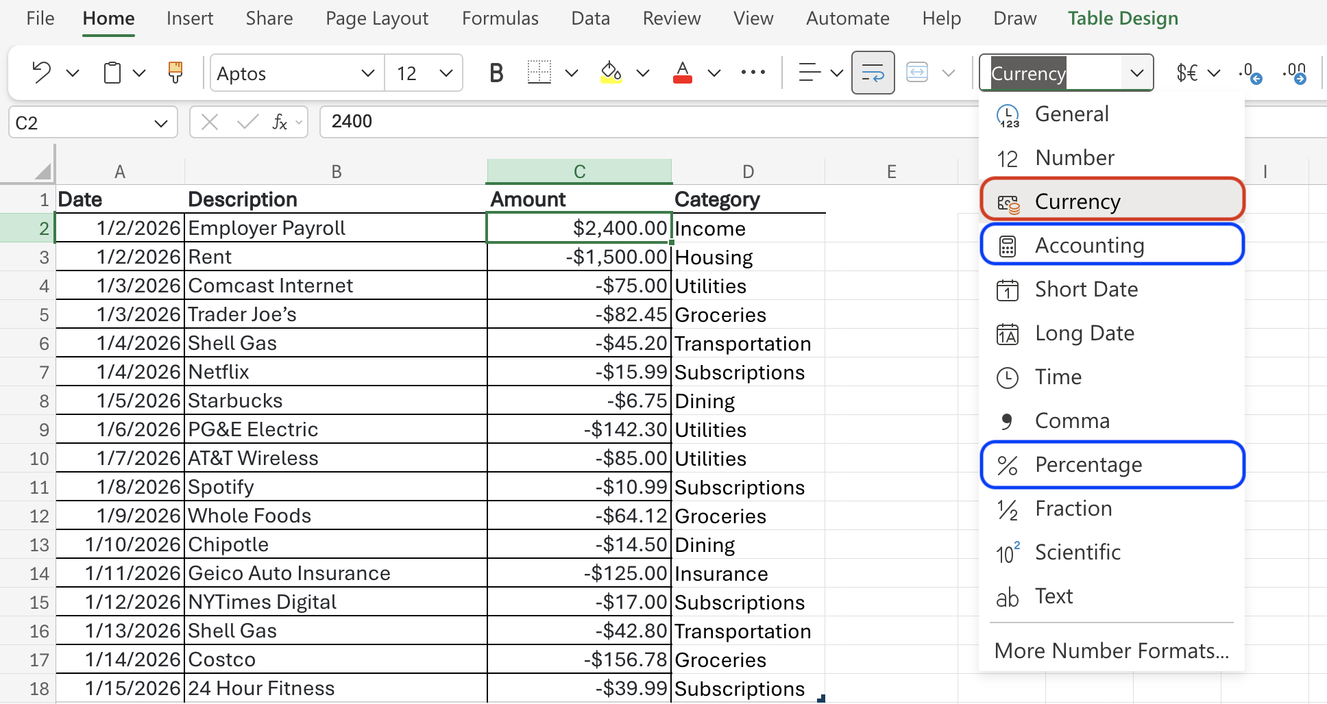
There are two options for money: Currency and Accounting.¹

Both fmt_dollar() and fmt_pct() follow the same convention: input is always a plain number, output is always a string. They are used throughout the remaining sections to clean up results.

4 Fixed-Cost Ratio

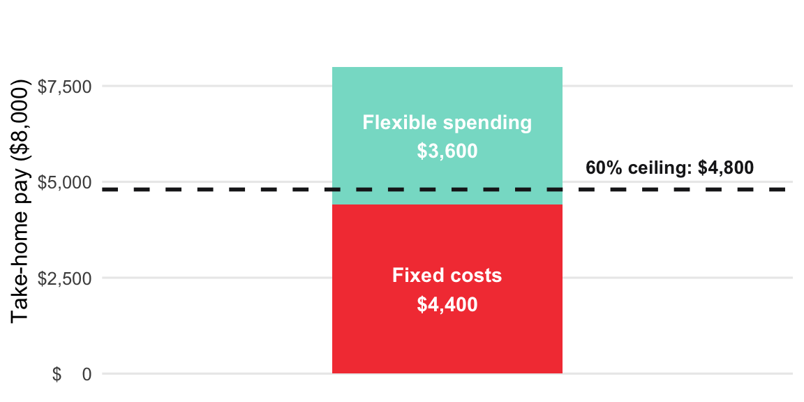
Fixed costs (rent, loans, insurance, utilities) should stay under ~60% of take-home pay.

Formula: Fixed-Cost Ratio = Fixed Costs ÷ Take-Home Pay × 100

Take-home pay divided into fixed costs and flexible spending ($8,000 total)

R

fixed_cost_ratio <- function(fixed_costs, take_home) {
  fixed_costs / take_home
}

fixed_cost_ratio(fixed_costs = 4400, take_home = 8000)
#> [1] 0.55

Python

def fixed_cost_ratio(fixed_costs, take_home):
    return fixed_costs / take_home

fixed_cost_ratio(fixed_costs=4400, take_home=8000)
#> 0.55

Excel

Enter fixed costs in A2, take-home in B2, then in C2:

=A2/B2

Format C2 as percentage (Home → %). For a percent string:

=TEXT(A2/B2, "0.0%")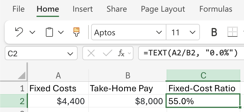

5 Using Pipes in R

The pipe operator (|>) passes the output of one function directly into the next function as its first argument, so the code reads left to right instead of inside out. We previously wrote the fmt_pct() function, so we can ‘pipe’ the output of fixed_cost_ratio() into fmt_pct() to get a formatted percentage string.

fixed_cost_ratio(fixed_costs = 4400, take_home = 8000) |> fmt_pct()

Read that as: compute the ratio, then format it as a percentage. The alternative without a pipe nests the calls and reads from the inside out, which is harder to follow.

fmt_pct(fixed_cost_ratio(fixed_costs = 4400, take_home = 8000))

When two steps always belong together, wrap them in a single function so callers only see one name.

fixed_cost_ratio <- function(fixed_costs, take_home) {
  ratio <- fixed_costs / take_home
    fmt_pct(ratio)
}

fixed_cost_ratio(fixed_costs = 4400, take_home = 8000)
#> [1] "55%"

This would also work:

fixed_cost_ratio <- function(fixed_costs, take_home) {
  fmt_pct(fixed_costs / take_home)
}

fixed_cost_ratio(fixed_costs = 4400, take_home = 8000)
#> [1] "55%"

Python has no native pipe operator. The equivalent is returning the result from fixed_cost_ratio() and passing this value to fmt_pct():

def fixed_cost_ratio(fixed_costs, take_home):
    ratio = fixed_costs / take_home
    return fmt_pct(ratio)

fixed_cost_ratio(fixed_costs=4400, take_home=8000)
#> '55.0%'

Python’s approach emphasizes explicit intermediate steps. Store the result of fixed_cost_ratio() in a variable (ratio), then pass it to fmt_pct(). This reads top-to-bottom and makes debugging easier since you can inspect intermediate values.

Both languages can call utility functions from within other functions; the key difference is that R’s pipe operator (|>) allows chaining without intermediate variables, while Python requires them or nested calls.

Read more about the pipe operator in R vs. Python.

6 Split Raise Strategy

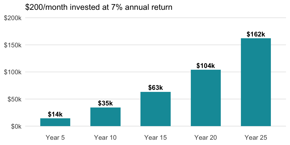
Split every raise: invest half, spend half. The future value of contributions formula shows how powerful this habit is.

Formula: FV = PMT × [((1 + r)^n − 1) ÷ r]

$200/month invested at 7% — value at each 5-year checkpoint

R

raise_invested_value <- function(monthly_raise, invest_share, rate, years) {
  contribution <- monthly_raise * invest_share
  monthly_rate <- rate / 12
  periods      <- years * 12
  (contribution * (((1 + monthly_rate)^periods - 1) / monthly_rate)) |>
    fmt_dollar()
}

Half of a $400/month raise, invested for 25 years at 7%:

raise_invested_value(monthly_raise = 400, invest_share = 0.5,
                     rate = 0.07, years = 25)
#> [1] "$162,014.34"

Python

def raise_invested_value(monthly_raise, invest_share, rate, years):
    contribution = monthly_raise * invest_share
    monthly_rate = rate / 12
    periods = years * 12
    fv = contribution * (((1 + monthly_rate) ** periods - 1) / monthly_rate)
    return fmt_dollar(fv)

Half of a $400/month raise, invested for 25 years at 7%:

raise_invested_value(monthly_raise=400, invest_share=0.5, rate=0.07, years=25)
#> '$162,014.34'

Excel

Use the built-in FV() function: FV(rate, nper, pmt)

• rate: monthly return = 7%/12
• nper: number of months = 25*12
• pmt: monthly contribution as a negative = -200

=FV(7%/12, 25*12, -200)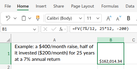

Footnotes

1. Read more about the differences between Currency and Accounting formats in Excel.