Investing Basics

1 Book Topics

• Compounding: interest earning interest; does the heavy lifting over long horizons; Rule of 72 — years to double ≈ 72 ÷ annual return %
• Risk vs. return: higher expected return = higher volatility; choose a level you can stick with through downturns
• Diversification: don’t bet on one company, sector, or country; broad index funds make diversification nearly free (Bogle)
• Real vs. nominal return: inflation silently erodes purchasing power; always think in real (inflation-adjusted) terms

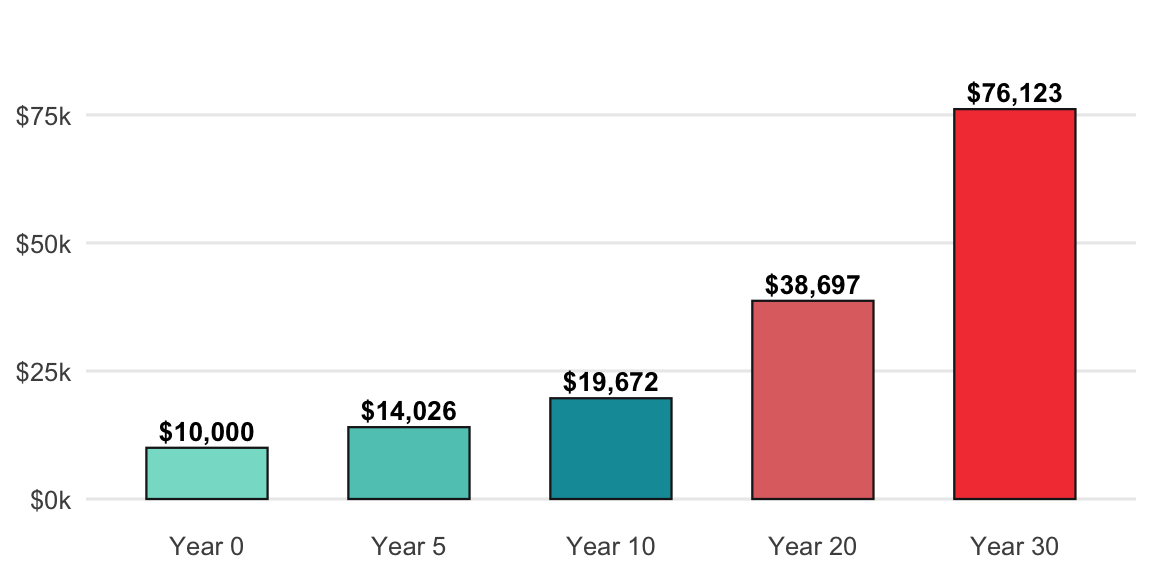
2 Future Value (Compounding)

A single lump sum growing at a constant rate.

Formula: FV = PV × (1 + r)^n

$10,000 growing at 7% — value at each checkpoint

R

future_value <- function(present_value, rate, years) {
  present_value * (1 + rate)^years
}

rule_of_72 <- function(annual_return_pct) {
  72 / annual_return_pct
}

future_value(present_value = 10000, rate = 0.07, years = 10)
#> [1] 19671.51
rule_of_72(annual_return_pct = 7)
#> [1] 10.28571

# vectorized across multiple horizons
data.frame(
  years = c(5, 10, 20, 30),
  value = future_value(10000, 0.07, c(5, 10, 20, 30))
)
#> # A tibble: 4 × 2
#>   years  value
#>   <dbl>  <dbl>
#> 1     5 14026.
#> 2    10 19672.
#> 3    20 38697.
#> 4    30 76123.

Python

import numpy as np

def future_value(present_value, rate, years):
    return present_value * (1 + rate) ** years

def rule_of_72(annual_return_pct):
    return 72 / annual_return_pct

print(future_value(present_value=10000, rate=0.07, years=10))
#> 19671.513572895663
print(rule_of_72(annual_return_pct=7))
#> 10.285714285714286

horizons = np.array([5, 10, 20, 30])
future_value(present_value=10000, rate=0.07, years=horizons)
#> array([14025.517307  , 19671.5135729 , 38696.84462486, 76122.55042662])

Excel

With present value in A2, rate in B2, years in C2:

=A2*(1+B2)^C2

Rule of 72 (rate as a percent in A2):

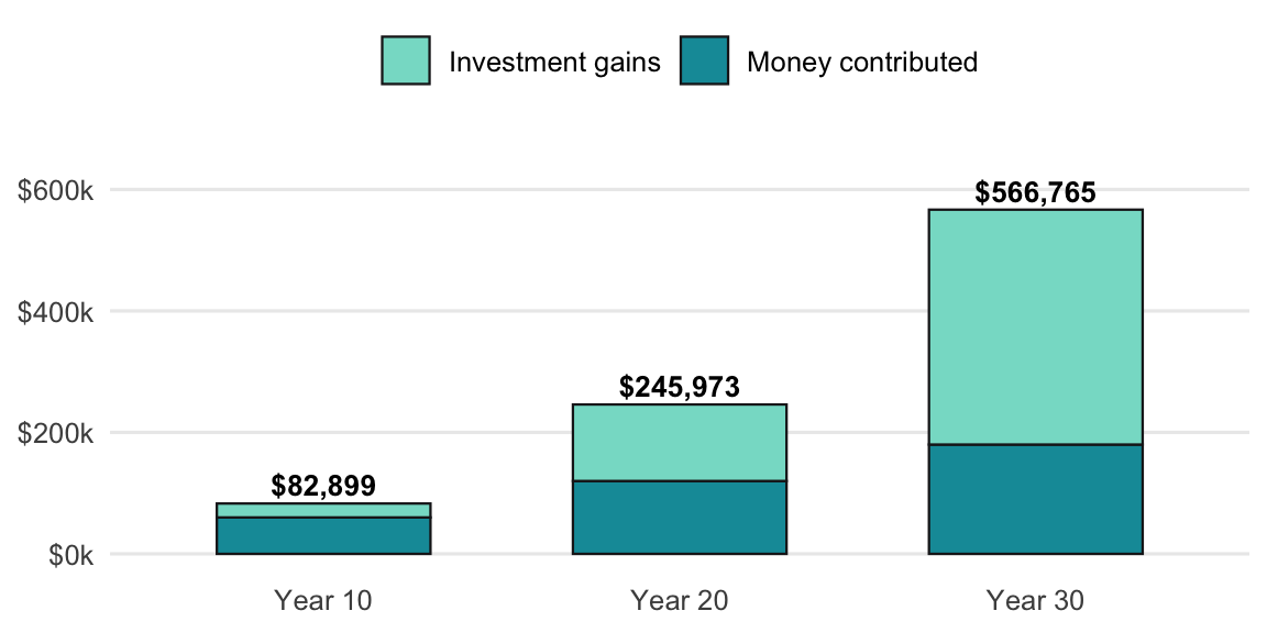
=72/A2

3 Future Value of Regular Contributions

Monthly investing builds wealth two ways: the money contributed and the returns on all prior contributions.

Formula: FV = PMT × [((1 + r)^n − 1) ÷ r]

$500/month contributions at 7% — contributed vs. gains

R

future_value_series <- function(contribution, rate, periods) {
  contribution * (((1 + rate)^periods - 1) / rate)
}

# $500/month for 30 years at 7% annual (monthly rate = 0.07/12)
future_value_series(contribution = 500, rate = 0.07 / 12, periods = 30 * 12)
#> [1] 609985.5

Python

def future_value_series(contribution, rate, periods):
    return contribution * (((1 + rate) ** periods - 1) / rate)

future_value_series(contribution=500, rate=0.07 / 12, periods=30 * 12)
#> 609985.4978879723

Excel

Use the built-in FV() function: FV(rate, nper, pmt)

• rate: monthly = 7%/12
• nper: months = 30*12
• pmt: monthly contribution as negative = -500

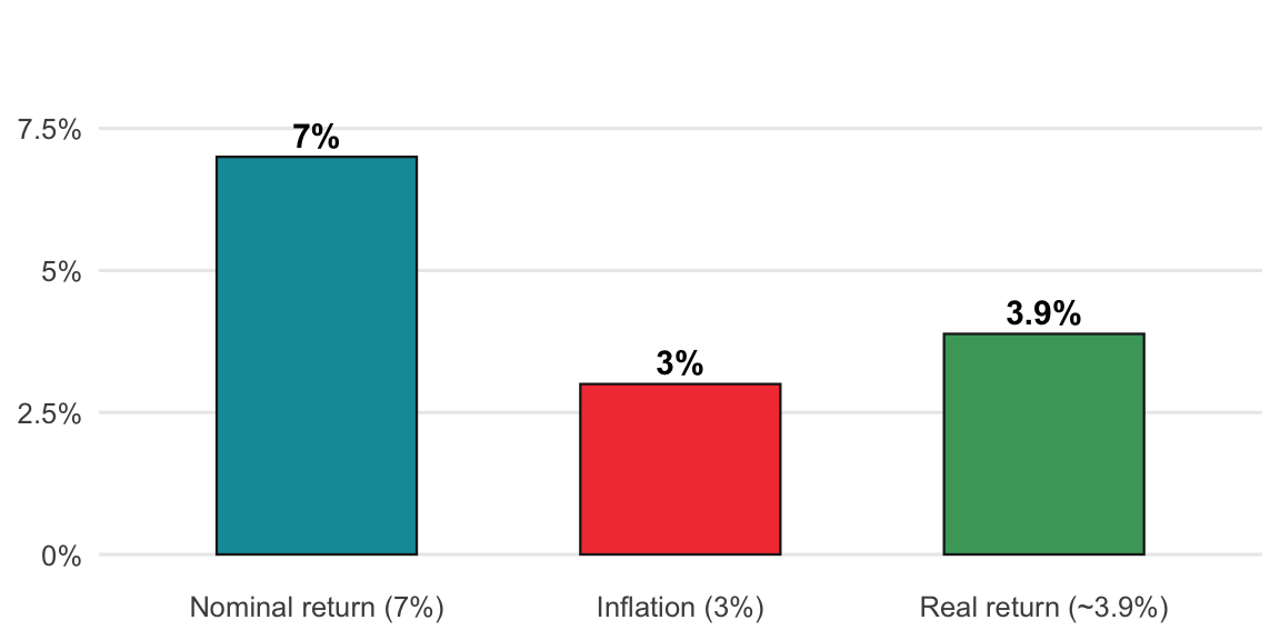
=FV(7%/12, 30*12, -500)

4 Real (Inflation-Adjusted) Return

Nominal returns overstate purchasing power gains; inflation takes its slice every year.

Formula: Real Return = (1 + nominal) ÷ (1 + inflation) − 1

Nominal return, inflation, and real return

R

real_return <- function(nominal, inflation) {
  (1 + nominal) / (1 + inflation) - 1
}

real_return(nominal = 0.07, inflation = 0.03)
#> [1] 0.03883495

Python

def real_return(nominal, inflation):
    return (1 + nominal) / (1 + inflation) - 1

real_return(nominal=0.07, inflation=0.03)
#> 0.03883495145631066

Excel

With nominal rate in A2 and inflation in B2:

=(1+A2)/(1+B2)-1