install.packages('pak')
pak::pkg_install("rstudio/plumber")plumber
This solution is a more robust example using the plumber package. I’ve summarized the changes to our original API (along with the inclusion of the logger package) below.
APIs (refresher)
We covered APIs in lab 3. APIs (Application Programming Interfaces) are a little like placing an order in a restaurant:
%%{init: {'theme': 'base', 'themeVariables': {'fontFamily': 'monospace'}}}%%

sequenceDiagram
    participant Customer as Shiny App
    participant Waiter as API
    participant Kitchen as ML Model

    Customer->>Waiter: "I'd like a<br>prediction for<br>bill_length=45,<br>species=Adelie"
    Waiter->>Kitchen: Prepare data &<br>make prediction
    Kitchen->>Waiter: Prediction: 4180.8 grams
    Waiter->>Customer: Returns prediction
The process involves three steps:
- The Shiny app asks for predictions.
- The Plumber API takes the values selected in the UI (as requests), and returns predictions (as responses).
- It’s the ML Model that does the actual work of calculating the predictions.
Overview
This architecture is comprised of three scripts in two folders:
api/
R/api/
├── api.Rproj
├── mod-api.R
├── model.R
├── models/
│ └── penguin_model/
├── my-db.duckdb
├── plumber.R
├── README.md
├── renv/
└── renv.lock- 1
-
model.Rbuilds and stores the model used for the predictions.
- 2
-
plumber.Rbuilds and launches theplumberAPI.
app/
R/app/
├── app-api.R
├── app.Rproj
├── renv/
└── renv.lock- 1
-
mod-api.Rreads the stored model and launches avetiverAPI.
We’ll go over each file in detail in the sections below.
The model (model.R)
The model.R file contains the necessary packages and functions to build the linear model we’re going to use to make the predictions from our Shiny app.1
show/hide model.R
library(palmerpenguins)
library(duckdb)
library(DBI)
library(dplyr)
library(vetiver)
library(pins)
con <- DBI::dbConnect(duckdb::duckdb(), "my-db.duckdb")
duckdb::duckdb_register(con, "penguins_raw", palmerpenguins::penguins)
DBI::dbExecute(
con,
"CREATE OR REPLACE TABLE penguins AS SELECT * FROM penguins_raw"
)
df <- DBI::dbGetQuery(
con,
"SELECT bill_length_mm, species, sex, body_mass_g
FROM penguins
WHERE body_mass_g IS NOT NULL
AND bill_length_mm BETWEEN 30 AND 60
AND sex IS NOT NULL
AND species IS NOT NULL"
)
DBI::dbDisconnect(con)
model <- lm(body_mass_g ~ bill_length_mm + species + sex, data = df)
v <- vetiver::vetiver_model(
model,
model_name = "penguin_model",
description = "Linear model predicting penguin body mass from bill length, species, and sex",
save_prototype = TRUE
)
model_board <- pins::board_folder("./models")
vetiver::vetiver_pin_write(model_board, v)- 1
- Load packages.
- 2
-
Use
DBIto connect toduckdb.
- 3
-
Register the penguins data.frame directly with
duckdb.
- 4
-
Create persistent table.
- 5
- Query and filter penguins data
- 6
-
Disconnect from database
- 7
-
Train the model. Unlike our previous example, we’ll use the original categorical variables and let R handle the dummy variable creation automatically.
- 8
-
Create
vetivermodel. - 9
-
Save the expected input format
- 10
- Write model to board
%%{init: {'theme': 'base', 'themeVariables': {'fontFamily': 'monospace'}}}%%

graph LR
    subgraph Training["<strong>Model Training</strong>"]
        ModelR("<strong>model.R</strong>")
        DuckDB("DuckDB <br> (as <strong>my-db.duckdb</strong>)")
        PinBoard("Pin Board<br><strong>models/penguin_model/</strong>")

        ModelR -->|"<em>loads data from</em>"| DuckDB
        ModelR -->|"<em>trains lm() model</em>"| LM("Linear Model")
        LM -->|"<em>wrapped by</em>"| Vetiver("Vetiver Model")
        Vetiver -->|"<em>saved to</em>"| PinBoard
    end
    style Training fill:#fbf7ec,stroke:#5B8C5A,color:#1B2A41
    style ModelR fill:#5B8C5A,stroke:#000000,stroke-width:1px,color:#ffffff
    style DuckDB fill:#5B8C5A,stroke:#000000,stroke-width:1px,color:#ffffff
    style LM fill:#D2562B,stroke:#000000,stroke-width:1px,color:#ffffff
    style Vetiver fill:#D2562B,stroke:#000000,stroke-width:1px,color:#ffffff
    style PinBoard fill:#2A6F77,stroke:#000000,stroke-width:1px,color:#ffffff
Running model.R creates the models/ directory and the duckdb database file:2
├── models
│ └── penguin_model
│ └── 20251005T062750Z-74445
│ ├── data.txt
│ └── penguin_model.rds
└── my-db.duckdb- 1
-
models/directory for the model
- 2
-
Local
duckdbdatabase
- 3
- The name of the model board (i.e., board subfolder)
- 4
-
Version timestamp + random ID
- 5
-
The
data.txtfile contains metadata about the pin
- 6
-
penguin_model.rdsis the serialized vetiver model
models includes a model_name from vetiver_model(), and we’ve add a description to accompany the metadata. data.txt stores metadata on the model:
readLines("models/penguin_model/20251005T062750Z-74445/data.txt") |>
  sprintf() |> noquote()
#  [1] file: penguin_model.rds
#  [2] file_size: 16401
#  [3] pin_hash: 7444544ac5799626
#  [4] type: rds
#  [5] title: 'penguin_model: a pinned list'
#  [6] description: Linear model predicting penguin body mass from bill length, species,
#  [7]   and sex
#  [8] tags: ~
#  [9] urls: ~
# [10] created: 20251005T062750Z
# [11] api_version: 1
# [12] user:
# [13]   required_pkgs: ~
# [14]   renv_lock: ~
The model is stored in the penguin_model.rds file, and we can see it contains the model and prototype.
v <- readRDS("models/penguin_model/20251005T062750Z-74445/penguin_model.rds")
str(v, max.level = 1)
# List of 2
#  $ model    :List of 13
#   ..- attr(*, "class")= chr [1:2] "butchered_lm" "lm"
#   ..- attr(*, "butcher_disabled")= chr [1:3] "print()" "summary()" "fitted()"
#  $ prototype:Classes ‘tbl_df’, ‘tbl’ and 'data.frame':    0 obs. of  3 variables:
model
This is our trained linear model.3
v$model
# Call:
# dummy_call()
#
# Coefficients:
#      (Intercept)    bill_length_mm  speciesChinstrap     speciesGentoo           sexmale
#          2169.27             32.54           -298.77           1094.87            547.37
If we dig a little deeper, we can see lm() object with coefficients, residuals, etc.
show/hide model structure
str(v$model, max.level = 1, list.len = 12)
# List of 13
#  $ coefficients : Named num [1:5] 2169.3 32.5 -298.8 1094.9 547.4
#   ..- attr(*, "names")= chr [1:5] "(Intercept)" "bill_length_mm"  ...
#  $ residuals    : Named num [1:333] -238.8 345.5 -230.5 86.6 -345.3 ...
#   ..- attr(*, "names")= chr [1:333] "1" "2" "3" "4" ...
#  $ effects      : Named num [1:333] -76772 8648 -9251 -2929 -3901 ...
#   ..- attr(*, "names")= chr [1:333] "(Intercept)" "bill_length_mm" ...
#  $ rank         : int 5
#  $ fitted.values: num(0)
#  $ assign       : int [1:5] 0 1 2 2 3
#  $ qr           :List of 5
#   ..- attr(*, "class")= chr "qr"
#  $ df.residual  : int 328
#  $ contrasts    :List of 2
#  $ xlevels      :List of 2
#  $ call         : language dummy_call()
#  $ terms        :Classes 'butchered_terms', 'terms', 'formula'  language body_mass_g ~ bill_length_mm + species + sex
#   .. ..- attr(*, "variables")= language list(body_mass_g, bill_length_mm, species, sex)
#   .. ..- attr(*, "factors")= int [1:4, 1:3] 0 1 0 0 0 0 1 0 0 0 ...
#   .. .. ..- attr(*, "dimnames")=List of 2
#   .. ..- attr(*, "term.labels")= chr [1:3] "bill_length_mm" "species" "sex"
#   .. ..- attr(*, "order")= int [1:3] 1 1 1
#   .. ..- attr(*, "intercept")= int 1
#   .. ..- attr(*, "response")= int 1
#   .. ..- attr(*, ".Environment")=<environment: base>
#   .. ..- attr(*, "predvars")= language list(body_mass_g, bill_length_mm, species, sex)
#   .. ..- attr(*, "dataClasses")= Named chr [1:4] "numeric" "numeric" "factor" "factor"
#   .. .. ..- attr(*, "names")= chr [1:4] "body_mass_g" "bill_length_mm" "species" "sex"
#   [list output truncated]
#  - attr(*, "class")= chr [1:2] "butchered_lm" "lm"
#  - attr(*, "butcher_disabled")= chr [1:3] "print()" "summary()" "fitted()"
prototype
The prototype is the expected input format, including the required column names, the expected data types (numeric, factor), and the factor levels (Adelie, Chinstrap, Gentoo or female, male).
str(v$prototype)
# Classes ‘tbl_df’, ‘tbl’ and 'data.frame': 0 obs. of  3 variables:
#  $ bill_length_mm: num
#  $ species       : Factor w/ 3 levels "Adelie","Chinstrap",..:
#  $ sex           : Factor w/ 2 levels "female","male":
The API (plumber.R)
The code below is from the plumber.R file. I’ve removed some of the print() and cat() statements to focus on each step.4
Load model
library(vetiver)
library(pins)
library(plumber)
library(jsonlite)
model_board <- pins::board_folder("models/")
v <- vetiver::vetiver_pin_read(model_board, "penguin_model")- 1
-
Packages
- 2
-
Connect to model board
- 3
- Read pinned vetiver model
Prepare prediction data
When R builds a linear model using categorical variables, it will convert these values to factors. However, JSON doesn’t have factors – only strings. The prep_pred_data() function bridges the gap by converting species and sex to factors.
prep_pred_data <- function(input_data) {
  species_levels <- levels(v$prototype$species)
  sex_levels <- levels(v$prototype$sex)

  data.frame(
    bill_length_mm = as.numeric(input_data$bill_length_mm),
    species = factor(input_data$species, levels = species_levels),
    sex = factor(input_data$sex, levels = sex_levels),
    stringsAsFactors = FALSE
  )
}
This function uses the prototype stored in the vetiver model to get the correct factor levels for species and sex.
%%{init: {'theme': 'base', 'themeVariables': {'fontFamily': 'monospace'}}}%%

graph TB
    subgraph JSON["JSON from Shiny"]
        J1("species: 'Adelie'<br>(string)")
        J2("sex: 'male'<br>(string)")
    end

    subgraph Model["Model Expects"]
        M1("species: factor<br>(with levels)")
        M2("sex: factor<br>(with levels)")
    end

    subgraph Helper["Helper Function"]
        H("prep_pred_data()")
    end

    J1 & J2 --> Helper
    Helper --> M1 & M2
    style JSON fill:#fbf7ec,stroke:#5B8C5A,color:#1B2A41
    style Model fill:#fbf7ec,stroke:#2A6F77,color:#1B2A41
    style Helper fill:#fbf7ec,stroke:#D2562B,color:#1B2A41
    style J1 fill:#5B8C5A,stroke:#000000,stroke-width:1px,color:#ffffff
    style J2 fill:#5B8C5A,stroke:#000000,stroke-width:1px,color:#ffffff
    style H fill:#D2562B,stroke:#000000,stroke-width:1px,color:#ffffff
    style M1 fill:#2A6F77,stroke:#000000,stroke-width:1px,color:#ffffff
    style M2 fill:#2A6F77,stroke:#000000,stroke-width:1px,color:#ffffff
Handler functions
Each handler specializes in different types of requests. We’re going to break these into four categories: health, model info, documentation, and predictions.
Health
The first two plumber functions in our plumber.R file are for checking the health of the API.
/ping
The first function is simple health check–it sends a ping to see if the API is running:
show/hide handle_ping()
#* Basic health check
#*
#* Simple endpoint to verify the API is running. Returns a minimal response
#* with status and timestamp.
#*
#* @get /ping
#*
#* @serializer json
#*
handle_ping <- function() {
  list(
    status = "alive",
    timestamp = Sys.time()
  )
}
This can be used to ensure API is up. We can test this from the Terminal with curl:
curl http://127.0.0.1:8080/ping{
"status": [
"alive"
],
"timestamp": [
"2025-10-08 08:31:51"
]
}/health
The handle_health() function will check the model version, R version, etc.
show/hide handle_health()
#* Detailed health check
#*
#* Extended health check that includes model metadata, version
#* information, and R version.
#*
#* @get /health
#*
#* @serializer json
#*
handle_health <- function() {
  list(
    status = "healthy",
    timestamp = Sys.time(),
    model_name = v$model_name,
    model_version = v$metadata$version,
    r_version = R.version.string
  )
}
This is useful for monitoring and debugging. Below is an example using curl.
curl http://127.0.0.1:8080/health{
"status": [
"healthy"
],
"timestamp": [
"2025-10-08 08:38:29"
],
"model_name": [
"penguin_model"
],
"model_version": [
"20251005T062750Z-74445"
],
"r_version": [
"R version 4.5.1 (2025-06-13)"
]
}Model Info
The functions below return the information on what to send in API requests.
/model-prototype
handle_model_prototype() will return the expected format for all requests.
show/hide handle_model_prototype()
#* Get model prototype information
#*
#* Returns the expected input format for the model, including
#* data types and factor levels.
#*
#* @get /model-prototype
#*
#* @serializer json
#*
handle_model_prototype <- function() {
  list(
    prototype = list(
      bill_length_mm = "numeric",
      species = list(
        type = "factor",
        levels = levels(v$prototype$species)
      ),
      sex = list(
        type = "factor",
        levels = levels(v$prototype$sex)
      )
    ),
    model_class = class(v$model)
  )
}
This is useful for clients to understand what data to send. Below is an example of handle_model_prototype() using curl:
curl http://127.0.0.1:8080/model-prototypeWe can see the response includes prototype and model_class:
show/hide JSON response from model-prototype
{
  "prototype": {
    "bill_length_mm": [
      "numeric"
    ],
    "species": {
      "type": [
        "factor"
      ],
      "levels": [
        "Adelie",
        "Chinstrap",
        "Gentoo"
      ]
    },
    "sex": {
      "type": [
        "factor"
      ],
      "levels": [
        "female",
        "male"
      ]
    }
  },
  "model_class": [
    "butchered_lm",
    "lm"
  ]
}
/model-info
We can get information about the model with handle_model_info(). This endpoint returns the metadata on our model.
show/hide handle_model_info()
#* Get model information and metadata
#*
#* Returns comprehensive information about the deployed model including
#* name, version, creation date, and required packages.
#*
#* @get /model-info
#*
#* @serializer json
#*
handle_model_info <- function() {
  list(
    model_name = v$model_name,
    model_class = class(v$model)[1],
    version = v$metadata$version,
    created = v$metadata$created,
    required_pkgs = v$metadata$required_pkgs,
    description = v$description %||% "No description available"
  )
}
Below is an example using curl:
curl http://127.0.0.1:8080/model-infoWe can see this returns the model name, class, version, and description.
show/hide JSON response from model-info
{
  "model_name": [
    "penguin_model"
  ],
  "model_class": [
    "butchered_lm"
  ],
  "version": [
    "20251005T062750Z-74445"
  ],
  "created": {},
  "required_pkgs": {},
  "description": [
    "Linear model predicting penguin body mass from bill length, species, and sex"
  ]
}
Documentation
We will include specifications for the API endpoint and an example of a prediction.
/input-schema
The handle_input_schema() function returns the model schema and example prediction values (properly formatted).
Code
#* Get input schema and example
#*
#* Returns documentation about the expected input fields, including
#* types, descriptions, valid values, and an example request.
#*
#* @get /input-schema
#*
#* @serializer json
#*
handle_input_schema <- function() {
  list(
    required_fields = list(
      bill_length_mm = list(
        type = "numeric",
        description = "Bill length in millimeters",
        range = c(30, 60)
      ),
      species = list(
        type = "string (converted to factor)",
        description = "Penguin species",
        valid_values = levels(v$prototype$species)
      ),
      sex = list(
        type = "string (converted to factor)",
        description = "Penguin sex",
        valid_values = levels(v$prototype$sex)
      )
    ),
    example = list(
      bill_length_mm = 45.5,
      species = "Gentoo",
      sex = "male"
    )
  )
}
When we use curl, we can see the response includes required_fields and the example:
curl http://127.0.0.1:8080/input-schemashow/hide JSON response from input-schema
{
  "required_fields": {
    "bill_length_mm": {
      "type": [
        "numeric"
      ],
      "description": [
        "Bill length in millimeters"
      ],
      "range": [
        30,
        60
      ]
    },
    "species": {
      "type": [
        "string (converted to factor)"
      ],
      "description": [
        "Penguin species"
      ],
      "valid_values": [
        "Adelie",
        "Chinstrap",
        "Gentoo"
      ]
    },
    "sex": {
      "type": [
        "string (converted to factor)"
      ],
      "description": [
        "Penguin sex"
      ],
      "valid_values": [
        "female",
        "male"
      ]
    }
  },
  "example": {
    "bill_length_mm": [
      45.5
    ],
    "species": [
      "Gentoo"
    ],
    "sex": [
      "male"
    ]
  }
}
Predictions
The primary prediction endpoint is stored in the handle_predict(). I’ve also included functions performing predictions with input validation and more than one prediction at a time.
/predict
The main prediction endpoint is stored in handle_predict(). I’ve removed the cat(), print(), and str() function calls to focus on each step.
show/hide handle_predict()
#* Predict penguin body mass
#*
#* Main prediction endpoint that accepts penguin characteristics and returns
#* predicted body mass in grams. Supports both single predictions and batch
#* predictions (multiple penguins in one request).
#*
#* @post /predict
#*
#* @serializer json
#*
handle_predict <- function(req, res) {
result <- tryCatch({
body <- jsonlite::fromJSON(req$postBody)
if (is.list(body) && !is.data.frame(body)) {
body <- as.data.frame(body)
}
pred_data <- prep_pred_data(body)
prediction <- predict(v, pred_data)
if (is.data.frame(prediction) && ".pred" %in% names(prediction)) {
response <- list(.pred = prediction$.pred)
} else if (is.numeric(prediction)) {
response <- list(.pred = as.numeric(prediction))
} else {
response <- list(.pred = as.numeric(prediction))
}
return(response)
}, error = function(e) {
cat("Error message:", conditionMessage(e), "\n")
print(e)
res$status <- 500
return(
list(
error = conditionMessage(e),
timestamp = as.character(Sys.time())
)
)
})
return(result)
}- 1
-
Parse JSON.
- 2
- Handle both single prediction and batch.
- 3
-
Prep data (convert strings to factors).
- 4
-
Make prediction.
- 5
- Handle different return types from vetiver.
- 6
-
Return response.
- 7
- Error handling.
The diagram below illustrates how data is transformed between requests and responses.
%%{init: {'theme': 'base', 'themeVariables': {'fontFamily': 'monospace'}}}%%

graph TB
    JSON("JSON String:<br>'{'bill_length_mm':45,...}'")

    JSON -->|"<em>fromJSON()</em>"| List("R List:<br>list(bill_length_mm=45,...)")

    List -->|"<em>as.data.frame()</em>"| DF("Data Frame:<br>1 row × 3 columns")

    DF -->|"<em>prep_pred_data()</em>"| Factors("Proper Types:<br>numeric + factors")

    Factors -->|"<em>predict</em>"| Result("Number:<br>4180.797")

    Result -->|"<em>list</em>"| Response("JSON Response:<br>{'.pred':[4180.797]}")

    style JSON fill:#5B8C5A,stroke:#000000,stroke-width:1px,color:#ffffff
    style List fill:#D2562B,stroke:#000000,stroke-width:1px,color:#ffffff
    style DF fill:#D2562B,stroke:#000000,stroke-width:1px,color:#ffffff
    style Factors fill:#D2562B,stroke:#000000,stroke-width:1px,color:#ffffff
    style Result fill:#2A6F77,stroke:#000000,stroke-width:1px,color:#ffffff
    style Response fill:#2A6F77,stroke:#000000,stroke-width:1px,color:#ffffff
In the Terminal, we can send values for bill length, species, and sex using curl:
curl -X POST http://127.0.0.1:8080/predict \
  -H "Content-Type: application/json" \
  -d '{"bill_length_mm": 45, "species": "Adelie", "sex": "male"}'
This returns a simple JSON list with the prediction:
{
  ".pred": [
    4180.7965
  ]
}
In the R console, we see the output with all the cat(), print(), and str() function calls:
show/hide the R Console prediction summary
=== /predict called ===
Raw body: {"bill_length_mm": 45, "species": "Adelie", "sex": "male"}
Parsed body:
$bill_length_mm
[1] 45

$species
[1] "Adelie"

$sex
[1] "male"

Prepared data:
  bill_length_mm species  sex
1             45  Adelie male
'data.frame':   1 obs. of  3 variables:
 $ bill_length_mm: num 45
 $ species       : Factor w/ 3 levels "Adelie","Chinstrap",..: 1
 $ sex           : Factor w/ 2 levels "female","male": 2
Calling predict...
Prediction result:
       1
4180.797
Prediction class: numeric
Response:
$.pred
[1] 4180.797

=== /predict complete ===
/predict-validated
handle_predict_validated() performs the same action as handle_predict(), but all of the input values are validated before the prediction is performed.
show/hide handle_predict_validated()
#* Predict with input validation
#*
#* Enhanced prediction endpoint that validates all inputs before making
#* predictions. Returns detailed error messages if validation fails.
#* Checks for:
#* - Required fields present
#* - Valid species (Adelie, Chinstrap, or Gentoo)
#* - Valid sex (male or female)
#* - Bill length in valid range (30-60mm)
#*
#* @post /predict-validated
#*
#* @serializer json
#*
handle_predict_validated <- function(req, res) {
result <- tryCatch({
body <- jsonlite::fromJSON(req$postBody)
required_fields <- c("bill_length_mm", "species", "sex")
missing_fields <- setdiff(required_fields, names(body))
if (length(missing_fields) > 0) {
res$status <- 400
return(list(
error = "Missing required fields",
missing = missing_fields,
hint = "Required fields: bill_length_mm, species, sex"
))
}
valid_species <- levels(v$prototype$species)
if (!body$species %in% valid_species) {
res$status <- 400
return(list(
error = "Invalid species",
provided = body$species,
valid_options = valid_species
))
}
valid_sex <- levels(v$prototype$sex)
if (!body$sex %in% valid_sex) {
res$status <- 400
return(list(
error = "Invalid sex",
provided = body$sex,
valid_options = valid_sex
))
}
if (!is.numeric(body$bill_length_mm) ||
body$bill_length_mm < 30 ||
body$bill_length_mm > 60) {
res$status <- 400
return(list(
error = "bill_length_mm must be numeric between 30 and 60",
provided = body$bill_length_mm,
valid_range = c(30, 60)
))
}
pred_data <- prep_pred_data(body)
prediction <- predict(v, pred_data)
list(
prediction = as.numeric(prediction),
input = body,
model_version = v$metadata$version,
timestamp = Sys.time()
)
}, error = function(e) {
cat("Error:", conditionMessage(e), "\n")
res$status <- 500
return(
list(
error = conditionMessage(e),
timestamp = as.character(Sys.time())
)
)
})
return(result)
}- 1
-
Collect response in JSON
- 2
-
Validate required fields
- 3
-
Check for missing fields
- 4
-
Validate species
- 5
-
Validate sex
- 6
-
Validate bill length
- 7
-
Prepare data
- 8
-
Make prediction
- 9
-
Prepare list
- 10
- Error handling
%%{init: {'theme': 'base', 'themeVariables': {'fontFamily': 'monospace'}}}%%

graph TD
    Start("Request<br>Received")

    Start --> Check1{All fields<br>present?}
    Check1 -->|No| Error1("❌ Return:<br>Missing fields error")
    Check1 -->|Yes| Check2{Species<br>valid?}

    Check2 -->|No| Error2("❌ Return:<br>Invalid species error")
    Check2 -->|Yes| Check3{Sex<br>valid?}

    Check3 -->|No| Error3("❌ Return:<br>Invalid sex error")
    Check3 -->|Yes| Check4{Bill length<br>30-60mm?}

    Check4 -->|No| Error4("❌ Return:<br>Out of range error")
    Check4 -->|Yes| Predict("Make Prediction")

    Predict --> Success("Return prediction<br>with metadata")

    style Start fill:#5B8C5A,stroke:#000000,stroke-width:1px,color:#ffffff
    style Check1 fill:#485466,stroke:#000000,stroke-width:1px,color:#ffffff
    style Check2 fill:#485466,stroke:#000000,stroke-width:1px,color:#ffffff
    style Check3 fill:#485466,stroke:#000000,stroke-width:1px,color:#ffffff
    style Check4 fill:#485466,stroke:#000000,stroke-width:1px,color:#ffffff
    style Error1 fill:#D2562B,stroke:#000000,stroke-width:1px,color:#ffffff
    style Error2 fill:#D2562B,stroke:#000000,stroke-width:1px,color:#ffffff
    style Error3 fill:#D2562B,stroke:#000000,stroke-width:1px,color:#ffffff
    style Error4 fill:#D2562B,stroke:#000000,stroke-width:1px,color:#ffffff
    style Predict fill:#5B8C5A,stroke:#000000,stroke-width:1px,color:#ffffff
    style Success fill:#2A6F77,stroke:#000000,stroke-width:1px,color:#ffffff
Below is an example of a valid request using the input validation:
curl -X POST http://127.0.0.1:8080/predict-validated \
  -H "Content-Type: application/json" \
  -d '{"bill_length_mm": 45, "species": "Adelie", "sex": "male"}'
Below is the validated prediction response.
{
  "prediction": [
    4180.7965
  ],
  "input": {
    "bill_length_mm": [
      45
    ],
    "species": [
      "Adelie"
    ],
    "sex": [
      "male"
    ]
  },
  "model_version": [
    "20251005T062750Z-74445"
  ],
  "timestamp": [
    "2025-10-08 14:04:44"
  ]
}
If we send an invalid species, the API will return error:
curl -X POST http://127.0.0.1:8080/predict-validated \
   -H "Content-Type: application/json" \
   -d '{"bill_length_mm": 45, "species": "Emperor", "sex": "male"}'
We can see the error includes the provided incorrect value.
{
  "error": [
    "Invalid species"
  ],
  "provided": [
    "Emperor"
  ],
  "valid_options": [
    "Adelie",
    "Chinstrap",
    "Gentoo"
  ]
}
/predict-batch
handle_predict_batch() lets us send more than one request to the API and receive multiple predictions. This request is slightly different because they must be arrays of the same length.
show/hide handle_predict_batch()
#* Batch predictions
#*
#* Predict body mass for multiple penguins in a single request.
#* Send arrays of values for each field.
#*
#* @post /predict-batch
#*
#* @serializer json
#*
handle_predict_batch <- function(req, res) {
result <- tryCatch({
body <- jsonlite::fromJSON(req$postBody)
if (!is.data.frame(body)) {
body <- as.data.frame(body)
}
pred_data <- prep_pred_data(body)
predictions <- predict(v, pred_data)
list(
predictions = as.numeric(predictions),
count = nrow(pred_data),
timestamp = Sys.time()
)
}, error = function(e) {
res$status <- 500
return(list(
error = conditionMessage(e),
timestamp = as.character(Sys.time())
))
})
return(result)
}- 1
-
Request body.
- 2
-
Ensure we have a
data.frame.
- 3
-
Prepare data.
- 4
-
Make predictions.
- 5
-
Create list with predictions, number of predictions, and a timestamp.
- 6
-
Error handling.
- 7
- Return prediction.
Below are three predictions:
1. bill_length_mm = 45, species = "Adelie", sex = "male"
2. bill_length_mm = 39, species = "Adelie", sex = "female"
3. bill_length_mm = 50, species = "Gentoo", sex = "male"
curl -X POST http://127.0.0.1:8080/predict-batch \
   -H "Content-Type: application/json" \
   -d '{
     "bill_length_mm": [45, 39, 50],
     "species": ["Adelie", "Adelie", "Gentoo"],
     "sex": ["male", "female", "male"]
   }'
The response contains the predictions, along the number of predictions sent/returned and the timestamp.
{
  "predictions": [
    4180.7965,
    3438.2083,
    5438.3484
  ],
  "count": [
    3
  ],
  "timestamp": [
    "2025-10-08 13:45:41"
  ]
}
The Router
The last bit of code in plumber.R builds a router object by registering HTTP endpoint handlers with a functional pipeline. The pipeline starts with pr(), which returns a plumber router object.
The router object is passed to pr_set_api_spec(), which is used to create machine-readable API documentation following the OpenAPI standard.
show/hide plumber router
app <- plumber::pr() |>
  # openapi specification
  pr_set_api_spec(function(spec) {
    spec$info$title <- "Penguin Mass Predictor API"
    spec$info$description <- "API for predicting penguin body mass using a linear regression model trained on the Palmer Penguins dataset. Deployed with vetiver for MLOps best practices."
    spec$info$version <- "1.0.0"
    spec$info$contact <- list(
      name = "API Support",
      email = "mjfrigaard@pm.me"
    )
    spec$info$license <- list(
      name = "MIT",
      url = "https://opensource.org/licenses/MIT"
    )
    spec
  })
%%{init: {'theme': 'base', 'themeVariables': {'fontFamily': 'monospace'}}}%%
graph LR
Function("<strong>pr_set_api_spec()</strong>")
Function --> Title("<code>title</code>:<br><em>'Penguin Mass Predictor API'</em>")
Function --> Desc("<code>description</code>:<br><em>'API for predicting...'</em>")
Function --> Version("<code>version</code>:<br><em>'1.0.0'</em>")
Function --> Contact("<code>contact</code>:<br>name, email")
Function --> License("<code>license</code>:<br>MIT")
Title & Desc & Version & Contact & License --> Swagger("<strong>Generates Interactive Docs<br>at /__docs__/</strong>")
style Function fill:#5B8C5A,stroke:#000000,stroke-width:1px,color:#ffffff
style Title fill:#485466,stroke:#000000,stroke-width:1px,color:#ffffff
style Desc fill:#485466,stroke:#000000,stroke-width:1px,color:#ffffff
style Version fill:#485466,stroke:#000000,stroke-width:1px,color:#ffffff
style Contact fill:#485466,stroke:#000000,stroke-width:1px,color:#ffffff
style License fill:#485466,stroke:#000000,stroke-width:1px,color:#ffffff
style Swagger fill:#2A6F77,stroke:#000000,stroke-width:1px,color:#ffffff
Now that we have a router object with specifications, we can add the endpoints.
Endpoints
Each pr_get() or pr_post() call adds a route mapping (URL pattern + HTTP method → handler function) to the router’s internal dispatch table. The pipe operator enables a fluent interface for sequential configuration.
The GET and POST endpoints are created with pr_get() and pr_post() and have the following arguments:
path: is the endpoint path in the API.handler: the handler function we wrote above.serializer: this function ’translating a generated R value into output that a remote user can understand.”5tags: these are the labels/headers our endpoints are organized under in the API.
GET Endpoints
The GET endpoints are linked to their function couterparts via the @get and @serializer tags:
show/hide plumber GET endpoints
  # GET endpoints
  pr_get(
    path = "/ping",
    handler = handle_ping,
    serializer = plumber::serializer_json(),
    tags = "Health"
  ) |>
  pr_get(
    path = "/health",
    handler = handle_health,
    serializer = plumber::serializer_json(),
    tags = "Health"
  ) |>
  pr_get(
    path = "/model-prototype",
    handler = handle_model_prototype,
    serializer = plumber::serializer_json(),
    tags = "Model Info"
  ) |>
  pr_get(
    path = "/model-info",
    handler = handle_model_info,
    serializer = plumber::serializer_json(),
    tags = "Model Info"
  ) |>
  pr_get(
    path = "/input-schema",
    handler = handle_input_schema,
    serializer = plumber::serializer_json(),
    tags = "Documentation"
  )
Route table after GET registrations:
| Path | Method | Handler | Purpose |
|---|---|---|---|
/ping |
GET | handle_ping() |
Quick health check |
/health |
GET | handle_health() |
Detailed status |
/model-prototype |
GET | handle_model_prototype() |
Input format specification |
/model-info |
GET | handle_model_info() |
Model metadata |
/input-schema |
GET | handle_input_schema() |
Field documentation |
POST Endpoints
The POST endpoints are linked to their function couterparts via the @post and @serializer tags:
show/hide plumber POST endpoints
  pr_post(
    path = "/predict",
    handler = handle_predict,
    serializer = plumber::serializer_json(),
    tags = "Predictions"
  ) |>
  pr_post(
    path = "/predict-validated",
    handler = handle_predict_validated,
    serializer = plumber::serializer_json(),
    tags = "Predictions"
  ) |>
  pr_post(
    path = "/predict-batch",
    handler = handle_predict_batch,
    serializer = plumber::serializer_json(),
    tags = "Predictions"
  )
Updated route table:
| Path | Method | Handler | Purpose |
|---|---|---|---|
/predict |
POST | handle_predict() |
Basic prediction |
/predict-validated |
POST | handle_predict_validated() |
Prediction with validation |
/predict-batch |
POST | handle_predict_batch() |
Multiple predictions |
The Server
The code above only configures and builds the plumber router. It remains dormant until we activate it with pr_run():
app |> plumber::pr_run(port = 8080, host = "127.0.0.1")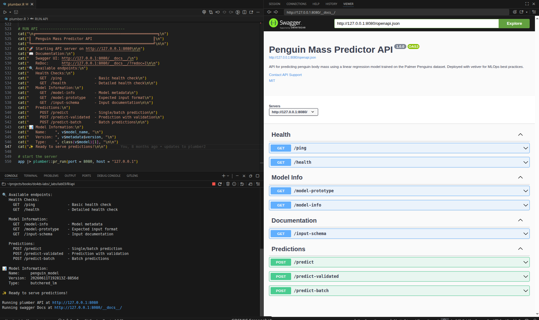
Now that the API is running, we can use a Shiny application to send values for penguin bill length, species, and sex and receive predictions.
%%{init: {'theme': 'base', 'themeVariables': {'fontFamily': 'monospace'}}}%%

sequenceDiagram
    participant Shiny as Shiny App
    participant Handler as handle_predict()
    participant Helper as prep_pred_data()
    participant Model as Linear Model

    Shiny->>Handler: POST /predict<br>{"bill_length_mm": 45,<br>"species": "Adelie",<br>"sex": "male"}

    Note over Handler: 1) Parse<br>JSON
    Handler->>Handler: jsonlite::fromJSON()

    Note over Handler: 2) Validate<br>& Convert
    Handler->>Helper: prep_pred_data()
    Helper-->>Handler: data.frame with factors

    Note over Handler: 3) Predict
    Handler->>Model: predict(v, data)
    Note over Model: y = β₀ +<br>β₁×bill_length +<br>β₂×species +<br>β₃×sex
    Model-->>Handler: 4180.797

    Note over Handler: 4) Format<br>response
    Handler->>Handler: list(.pred = 4180.797)

    Handler-->>Shiny: {"pred": [4180.797]}
The Shiny App (app-api.R)
The app-api.R file is a Shiny application that sends user input to the /predict endpoint and displays the returned prediction. It lives in the separate app/ directory.
The API URL is defined at the top of the file:
api_url <- "http://127.0.0.1:8080/predict"UI
show/hide UI
ui <- page_sidebar(
title = "Penguin Mass Predictor",
theme = bs_theme(bootswatch = "sketchy"),
sidebar = sidebar(
sliderInput(
inputId = "bill_length",
label = "Bill Length (mm)",
min = 30, max = 60, value = 45, step = 1
),
selectInput(
inputId = "sex",
label = "Sex",
choices = c("Male", "Female"),
selected = "Male"
),
selectInput(
inputId = "species",
label = "Species",
choices = c("Adelie", "Chinstrap", "Gentoo"),
selected = "Adelie"
),
actionButton(
inputId = "predict",
label = "Predict",
class = "btn-primary"
)
),
layout_columns(
card(
card_header("Penguin Parameters"),
card_body(verbatimTextOutput(outputId = "vals"))
),
card(
card_header("Predicted Mass"),
card_body(
value_box(
showcase_layout = "left center",
title = "Grams",
value = textOutput(outputId = "pred"),
showcase = bs_icon("graph-up"),
max_height = "200px",
min_height = "200px"
)
)
),
col_widths = c(7, 5)
)
)- 1
-
Sex choices are title-case (
"Male","Female");tolower()invals()converts them before sending to the API.
Reactive values
The vals() reactive builds a data.frame of the current inputs. tolower(input$sex) converts "Male" / "Female" to the lowercase strings the API prototype expects:
vals <- reactive({
data.frame(
bill_length_mm = input$bill_length,
species = input$species,
sex = tolower(input$sex)
)
})- 1
-
Species is passed as-is (
"Adelie","Chinstrap","Gentoo");prep_pred_data()in the API converts it to a factor. - 2
-
tolower()converts"Male"→"male"to match thesexfactor levels in the model prototype.
Predictions
The pred reactive sends vals() to the API and extracts the prediction:
show/hide pred reactive
pred <- reactive({
tryCatch({
showNotification("Predicting penguin mass...", type = "default", duration = 10)
request_data <- vals()
response <- httr2::request(api_url) |>
httr2::req_method("POST") |>
httr2::req_body_json(request_data, auto_unbox = FALSE) |>
httr2::req_perform() |>
httr2::resp_body_json()
showNotification("Prediction successful!", type = "default", duration = 10)
response$.pred[[1]]
}, error = function(e) {
error_msg <- conditionMessage(e)
if (grepl("Connection refused|couldn't connect", error_msg, ignore.case = TRUE)) {
user_msg <- "API not available - is the server running on port 8080?"
} else if (grepl("timeout|timed out", error_msg, ignore.case = TRUE)) {
user_msg <- "Request timed out - API may be overloaded"
} else {
user_msg <- paste("API Error:", substr(error_msg, 1, 50))
}
showNotification(paste("❌", user_msg), type = "warn", duration = 10)
paste("❌", user_msg)
})
}) |>
bindEvent(input$predict, ignoreInit = TRUE)- 1
-
vals()is assigned torequest_databefore the pipe so any reactive invalidation is captured once. - 2
-
auto_unbox = FALSEsends single values as JSON arrays (e.g.,[45]not45), which the/predicthandler’sas.data.frame(body)step handles correctly.
httr2 request/response pipeline
The five httr2 functions work as a pipeline, each building on the previous step:
%%{init: {'theme': 'base', 'themeVariables': {'fontFamily': 'monospace'}}}%%

graph TD
    ReqObj("request(url)") -->|"sets URL"| MethObj
    MethObj("req_method('POST')") -->|"sets verb"| BodyObj
    BodyObj("req_body_json(data)") -->|"attaches body"| PerfObj
    PerfObj("req_perform()") -->|"sends request"| RespObj
    RespObj("resp_body_json()") -->|"parses response"| Result("R list")

    style ReqObj fill:#5B8C5A,stroke:#000000,stroke-width:1px,color:#ffffff
    style MethObj fill:#D2562B,stroke:#000000,stroke-width:1px,color:#ffffff
    style BodyObj fill:#D2562B,stroke:#000000,stroke-width:1px,color:#ffffff
    style PerfObj fill:#D2562B,stroke:#000000,stroke-width:1px,color:#ffffff
    style RespObj fill:#D2562B,stroke:#000000,stroke-width:1px,color:#ffffff
    style Result fill:#2A6F77,stroke:#000000,stroke-width:1px,color:#ffffff
| Function | Role |
|---|---|
request(url) |
Creates a base request with the target URL |
req_method("POST") |
Sets the HTTP verb |
req_body_json(data, auto_unbox = FALSE) |
Serialises data as JSON arrays; sets Content-Type: application/json |
req_perform() |
Sends the assembled request; returns a response object |
resp_body_json() |
Parses the JSON response body into an R list |
Outputs
The server renders vals() and pred() to the UI:
output$vals <- renderPrint(vals())
output$pred <- renderText({
  prediction <- pred()
  if (is.numeric(prediction)) paste(round(prediction, 1), "grams") else prediction
})
Full app server
Below is the full app server:
show/hide full server
server <- function(input, output) {

  vals <- reactive({
    data.frame(
      bill_length_mm = input$bill_length,
      species = input$species,
      sex = tolower(input$sex)
    )
  })

  pred <- reactive({
    tryCatch({
      showNotification("Predicting penguin mass...", type = "default", duration = 10)

      request_data <- vals()

      response <- httr2::request(api_url) |>
        httr2::req_method("POST") |>
        httr2::req_body_json(request_data, auto_unbox = FALSE) |>
        httr2::req_perform() |>
        httr2::resp_body_json()

      showNotification("Prediction successful!", type = "default", duration = 10)

      response$.pred[[1]]

    }, error = function(e) {
      error_msg <- conditionMessage(e)

      if (grepl("Connection refused|couldn't connect", error_msg, ignore.case = TRUE)) {
        user_msg <- "API not available - is the server running on port 8080?"
      } else if (grepl("timeout|timed out", error_msg, ignore.case = TRUE)) {
        user_msg <- "Request timed out - API may be overloaded"
      } else {
        user_msg <- paste("API Error:", substr(error_msg, 1, 50))
      }

      showNotification(paste("❌", user_msg), type = "warn", duration = 10)
      paste("❌", user_msg)
    })
  }) |>
    bindEvent(input$predict, ignoreInit = TRUE)

  output$vals <- renderPrint(vals())
  output$pred <- renderText({
    prediction <- pred()
    if (is.numeric(prediction)) paste(round(prediction, 1), "grams") else prediction
  })
}

shinyApp(ui = ui, server = server)
Verify
In the Shiny app, when we click the Predict button, we see the response from the API (and our success notifications):
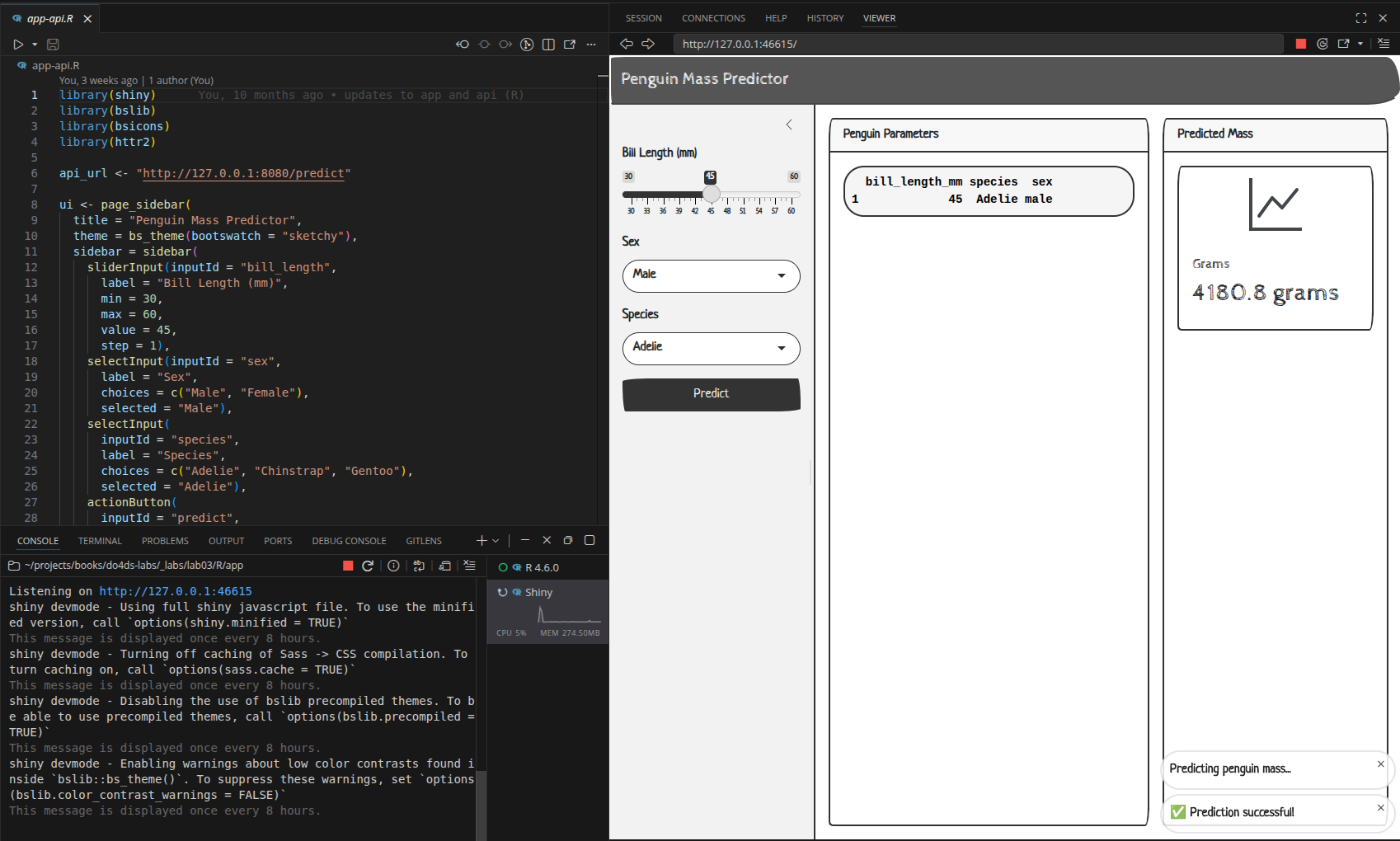
The full request/response flow from button click to displayed prediction:
%%{init: {'theme': 'base', 'themeVariables': {'fontFamily': 'monospace'}}}%%

sequenceDiagram
    participant Shiny as Shiny App
    participant Handler as handle_predict()
    participant Helper as prep_pred_data()
    participant Model as Linear Model

    Shiny->>Handler: POST /predict<br>{"bill_length_mm": 45,<br>"species": "Adelie",<br>"sex": "male"}

    Note over Handler: 1) Parse JSON
    Handler->>Handler: jsonlite::fromJSON()

    Note over Handler: 2) Validate<br>& Convert
    Handler->>Helper: prep_pred_data()
    Helper-->>Handler: data.frame with factors

    Note over Handler: 3) Predict
    Handler->>Model: predict(v, data)
    Note over Model: y = β₀ +<br>β₁×bill_length +<br>β₂×species +<br>β₃×sex
    Model-->>Handler: 4180.797

    Note over Handler: 4) Format<br>response
    Handler->>Handler: list(.pred = 4180.797)

    Handler-->>Shiny: {".pred": [4180.797]}
To keep environments self-contained and reproducible, initialize renv in each directory:
renv::init()We’ll cover this more in R App Logging.
View this file in the GitHub repo.↩︎
If you run this on your machine your folder will look slightly different because of the timestamp and random ID.↩︎
Read more about model versioning on the
vetiversite.↩︎Read ‘Model cards for transparent, responsible reporting’ for more information.↩︎
From the
plumberdocumentation on registered serializers.↩︎