Getting started • segtools

library(segtools)
library(dplyr)
library(vroom)
library(janitor)

Assume I have a .csv file with BGM and REF columns (like the one in the segtools inst/extdata/ folder:

test_data <- vroom::vroom(
  file = "https://bit.ly/3JwGoiP", delim = ",")
dplyr::glimpse(test_data)
#> Rows: 9,891
#> Columns: 2
#> $ BGM <dbl> 121, 212, 161, 191, 189, 104, 293, 130, 261, 147, 83, 132, 146, 24…
#> $ REF <dbl> 127, 223, 166, 205, 210, 100, 296, 142, 231, 148, 81, 131, 155, 25…

The segtools package can create the following outputs

Summary Tables

The summary tables rely on separate functions for each table.

Pairs table

seg_pairs_table() returns the pairs comparing BGM to REF

seg_pair_type_tbl(df = test_data)

Pair Type	Count
Total	9891
BGM < REF	4710
BGM = REF	479
BGM > REF	4702
REF > 600: Excluded from SEG Analysis	23
Total included in SEG Analysis	9868

MARD table

The MARD table requires two functions:

seg_risk_vars() to calculate the intermediate risk variables

risk_vars_tbl <- seg_risk_vars(df = test_data)

seg_mard_tbl() to calculate the Bias, MARD, CV, and lower/upper 95% CI

seg_mard_tbl(risk_vars_tbl)

Total	Bias	MARD	CV	Lower 95% Limit of Agreement	Upper 95% Limit of Agreement
9868	0.6%	7%	14.8%	-28.3%	29.6%

Risk grade table

seg_risk_grade_tbl() returns a table of risk grades

seg_risk_grade_tbl(risk_vars_tbl)

ID	Risk Grade	Number of Pairs	Percent	Risk Factor Range
1	A	9474	96%	0 - 0.5
2	B	349	3.5%	> 0.5 - 1.0
3	C	35	0.4%	> 1.0 - 2.0
4	D	10	0.1%	> 2.0 - 3.0
5	E	NA	NA	> 3.0

Risk category table

seg_risk_level_table() return a table of risk levels and categories

seg_risk_cat_tbl(risk_vars_tbl)

SEG Risk Level	SEG Risk Category	Number of Pairs	Percent
0	None	9474	96%
1	Slight, Lower	294	3%
2	Slight, Higher	55	0.6%
3	Moderate, Lower	24	0.2%
4	Moderate, Higher	11	0.1%
5	Severe, Lower	10	0.1%
6	Severe, Upper	NA	NA
7	Extreme	NA	NA

ISO range table

seg_iso_range_tbl() returns a table of compliance ranges

seg_iso_range_tbl(risk_vars_tbl)

ID	ISO range	N	Percent
1	<= 5% or 5 mg/dL	5328	54%
2	> 5 - 10% or mg/dL	2842	28.8%
3	> 10 - 15% or mg/dL	1050	10.6%
4	> 15 - 20% mg/dL	340	3.4%
5	> 20% or 20 mg/dL	308	3.1%

Compliant pairs table

seg_binom_tbl() returns a table binomial test for compliant pairs

seg_binom_tbl(risk_vars_tbl)

Compliant Pairs	Compliant Pairs %	Lower Bound for Acceptance	Lower Bound for Acceptance %	Result
9220	93.4%	9339	94.6%	93.4% < 94.6% - Does not meet BGM Surveillance Study Accuracy Standard

Graphs

segtools can also create the following graphs:

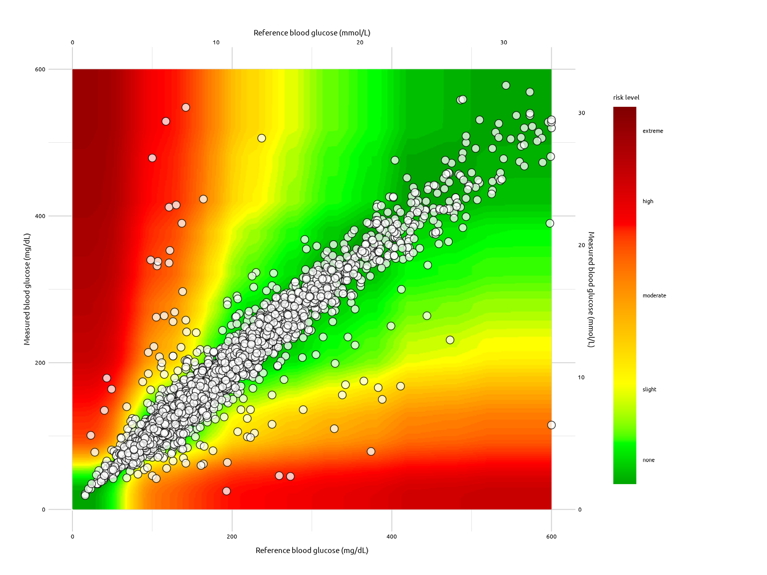
The SEG Graph

seg_graph(
  data = test_data,
  alpha_var = 3 / 4,
  size_var = 2.5,
  color_var = "#000000",
  fill_var = "#FFFFFF"
)

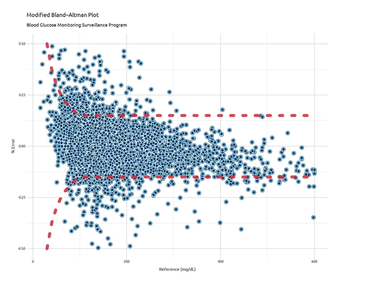
The Modified Bland-Altman Plot

source("../R/seg_modba_graph.R")
seg_modba_graph(data = test_data)