show/hide
years   <- 0:40
balance <- 10000 * (1.07)^years
plot(years, balance, type = "l",
     xlab = "Years", ylab = "Balance ($)",
     main = "$10,000 at 7% compounded annually")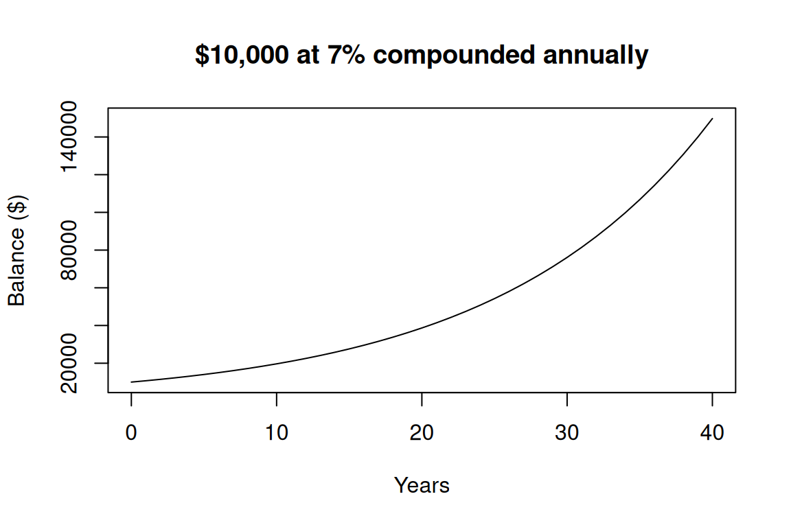
A short tour of the concepts behind every investment decision.
Compounding is interest earning interest. Over long horizons, it does the heavy lifting.
years <- 0:40
balance <- 10000 * (1.07)^years
plot(years, balance, type = "l",
xlab = "Years", ylab = "Balance ($)",
main = "$10,000 at 7% compounded annually")
years = list(range(0, 41))
balance = [10000 * (1.07) ** y for y in years]
balance[-1]  # ending balance after 40 years
#> 149744.57839206984
Formula: FV = PV × (1 + r)^n
Where: FV = future value, PV = present value, r = annual return, n = years
The shortcut you should memorize is the Rule of 72:
Years to double your money = 72 ÷ annual return %
At 7% return, money doubles every ~10 years. At 10%, every ~7 years. This single insight reframes every spending decision.
See Math for Investing Basics below for the future_value() and rule_of_72() functions in R and Python, plus the math for regular contributions and inflation-adjusted returns.
Higher expected return = higher expected volatility. Choose a level you can stick with through downturns, not just one that looks attractive on a spreadsheet.
Don’t bet on one company, one sector, or one country. Broad index funds make this nearly free.
Investing math is mostly one idea, compounding, applied in a few different ways. Each calculation below is written as an R and Python function, following the same pattern introduced in the Budgeting chapter.
In code, the ^ symbol (R) and ** symbol (Python) both mean “raise to the power of.” So (1 + 0.07)^10 means “1.07 multiplied by itself 10 times.”
Each bar below is the previous one multiplied by the same growth factor. The result is not a straight line — it curves upward because each year’s growth is applied to a larger base.
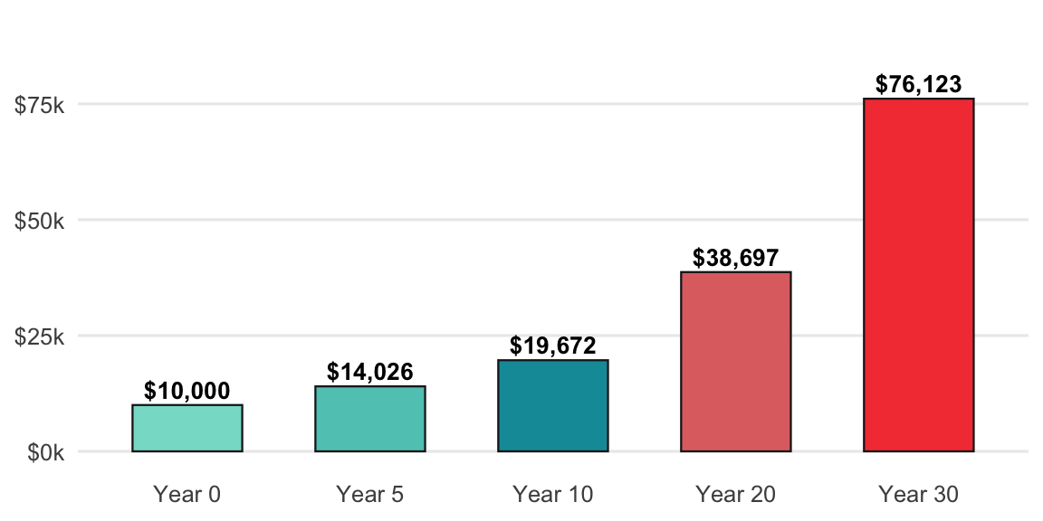
Multiplying by (1 + r) once gives next year’s value; multiplying by it n times gives the value after n years — that’s the formula.
Formula: FV = PV × (1 + r)^n
Where: FV = future value, PV = present value (today’s amount), r = annual return, n = years.
The companion shortcut is the Rule of 72: divide 72 by the return percentage to estimate how many years it takes your money to double.
Years to double ≈ 72 ÷ annual return %
Example: $10,000 at 7% for 10 years grows to ~$19,672, and at 7% money doubles roughly every 10 years.
future_value <- function(present_value, rate, years) {
  present_value * (1 + rate)^years
}

rule_of_72 <- function(annual_return_pct) {
  72 / annual_return_pct
}

# scalar: $10,000 at 7% for 10 years
future_value(present_value = 10000, rate = 0.07, years = 10)
#> [1] 19671.51

# how long until your money doubles at 7%?
rule_of_72(annual_return_pct = 7)
#> [1] 10.28571

# vectorized: same $10,000 at 7% across multiple horizons
data.frame(
  years = c(5, 10, 20, 30),
  value = future_value(present_value = 10000, rate = 0.07, years = c(5, 10, 20, 30))
)
#> # A tibble: 4 × 2
#>   years  value
#>   <dbl>  <dbl>
#> 1     5 14026.
#> 2    10 19672.
#> 3    20 38697.
#> 4 30 76123.import numpy as np
def future_value(present_value, rate, years):
return present_value * (1 + rate) ** years
def rule_of_72(annual_return_pct):
return 72 / annual_return_pct
# scalar: $10,000 at 7% for 10 years
print(future_value(present_value=10000, rate=0.07, years=10))
#> 19671.513572895663
# how long until your money doubles at 7%?
print(rule_of_72(annual_return_pct=7))
#> 10.285714285714286
# vectorized: numpy lets us pass an array of horizons in one call
horizons = np.array([5, 10, 20, 30])
future_value(present_value=10000, rate=0.07, years=horizons)
#> array([14025.517307 , 19671.5135729 , 38696.84462486, 76122.55042662])Investing a fixed amount every month builds wealth in two ways: the money you put in, and the growth earned on all previous contributions. The chart below separates these two layers so you can see when growth overtakes contributions.
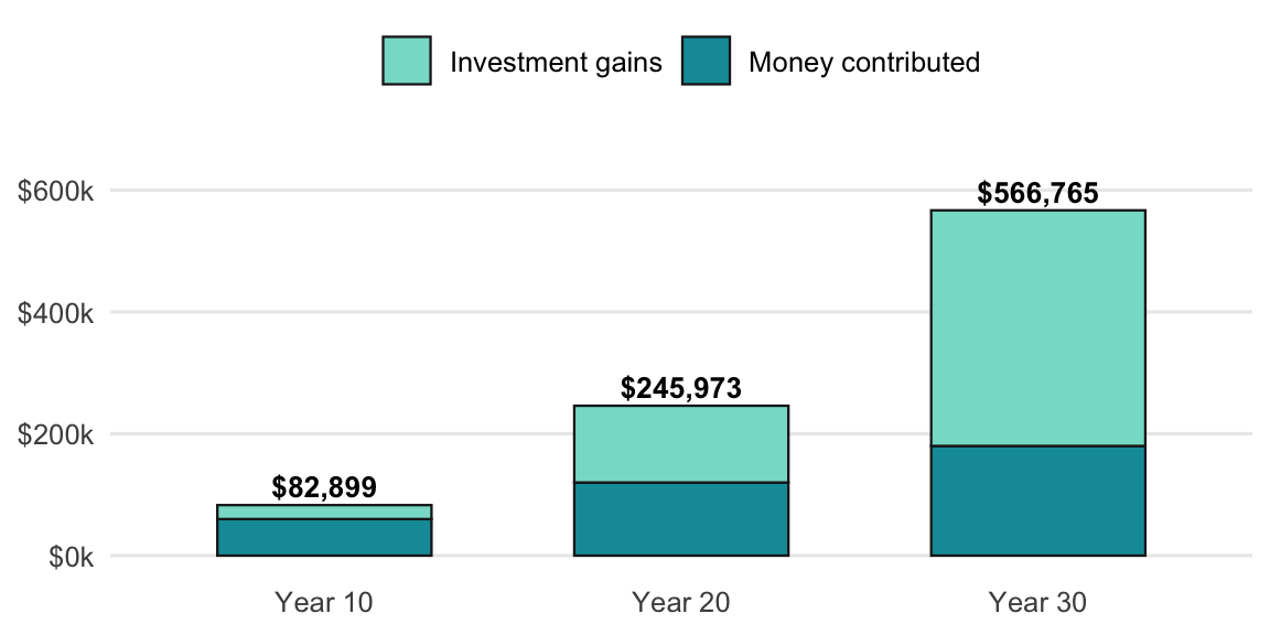
The formula sums all those contribution bars growing at different rates — the annuity formula collapses that sum into a single calculation.
Formula: FV = PMT × [((1 + r)^n − 1) ÷ r]
Where: PMT = the amount contributed each period, r = the return per period, n = the number of periods.
Example: $500/month for 30 years (360 months) at a 7% annual return (~0.583% per month) grows to ~$610,000, of which only $180,000 is money you actually put in.
future_value_series <- function(contribution, rate, periods) {
  contribution * (((1 + rate)^periods - 1) / rate)
}

# $500/month for 30 years at a 7% annual return (monthly rate = 0.07 / 12)
future_value_series(contribution = 500, rate = 0.07 / 12, periods = 30 * 12)
#> [1] 609985.5def future_value_series(contribution, rate, periods):
return contribution * (((1 + rate) ** periods - 1) / rate)
# $500/month for 30 years at a 7% annual return (monthly rate = 0.07 / 12)
future_value_series(contribution=500, rate=0.07 / 12, periods=30 * 12)
#> 609985.4978879723A 7% nominal return sounds good, but inflation is quietly shrinking the purchasing power of every dollar. The chart below shows the three quantities: the stated return, the inflation cost, and what actually remains.
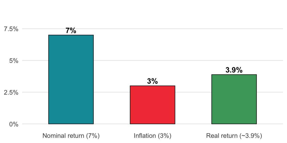
The real return is what’s left after inflation takes its slice — not a simple subtraction, but a ratio, because the percentages compound.
Formula: Real Return = (1 + nominal) ÷ (1 + inflation) − 1
Example: (1.07 ÷ 1.03) − 1 = ~3.88%, slightly less than the 4% you’d get by simple subtraction.
real_return <- function(nominal, inflation) {
  (1 + nominal) / (1 + inflation) - 1
}

# 7% nominal return against 3% inflation
real_return(nominal = 0.07, inflation = 0.03)
#> [1] 0.03883495def real_return(nominal, inflation):
return (1 + nominal) / (1 + inflation) - 1
# 7% nominal return against 3% inflation
real_return(nominal=0.07, inflation=0.03)
#> 0.03883495145631066