%%{init: {'theme': 'neutral', 'themeVariables': { 'fontFamily': 'monospace', "fontSize":"16px"}}}%%

flowchart TD
    AllDebt[Your Debts] --> Toxic[TOXIC DEBT<br>15-29% APR]
    AllDebt --> Moderate[MODERATE DEBT<br>5-10% APR]
    AllDebt --> Strategic[STRATEGIC DEBT<br>3-7% APR]

    Toxic --> CreditCards[Credit Cards<br>Payday Loans]
    Moderate --> CarLoans[Car Loans<br>Private Student Loans]
    Strategic --> Mortgages[Mortgages<br>Federal Student Loans]

    CreditCards --> Attack1[Attack Aggressively<br>Pay Off First]
    CarLoans --> Attack2[Pay Down Steadily<br>Avoid New Ones]
    Mortgages --> Attack3[Pay on Schedule<br>Invest the Difference]
    style AllDebt fill:#48a56a,color:#F5F2E8,stroke:#1C1C1E,stroke-width:2px
    style Toxic fill:#f44242,color:#F5F2E8,stroke:#1C1C1E,stroke-width:2px
    style Moderate fill:#f0cfcf,color:#1C1C1E,stroke:#1C1C1E,stroke-width:2px
    style Strategic fill:#86ddcd,color:#1C1C1E,stroke:#1C1C1E,stroke-width:2px
    style CreditCards fill:#f44242,color:#F5F2E8,stroke:#1C1C1E,stroke-width:2px
    style CarLoans fill:#0e9aa7,color:#F5F2E8,stroke:#1C1C1E,stroke-width:2px
    style Mortgages fill:#86ddcd,color:#1C1C1E,stroke:#1C1C1E,stroke-width:2px
    style Attack1 fill:#f44242,color:#F5F2E8,stroke:#1C1C1E,stroke-width:2px
    style Attack2 fill:#0e9aa7,color:#F5F2E8,stroke:#1C1C1E,stroke-width:2px
    style Attack3 fill:#86ddcd,color:#1C1C1E,stroke:#1C1C1E,stroke-width:2px
4 Managing Debt
Debt isn’t inherently good or bad; it’s a tool. Used wisely, it can accelerate wealth-building (think low-rate mortgages or strategic education). Used poorly, it can quietly destroy decades of financial progress. Let’s break down each type with evidence-based advice from Housel, Sethi, Bogle, and Ben Felix.
4.1 Where Debt Fits in the Financial Order of Operations
Brian Preston’s Financial Order of Operations (FOO), introduced in Budgeting, splits debt into two separate steps rather than treating it as one problem:
- Step 3 — High-interest debt. Credit cards, payday loans, and anything else in the toxic tier (see The Debt Hierarchy below) get paid off before you build a full emergency fund or invest beyond an employer match. The rate is simply too punishing to justify waiting.
- Step 9 — Low-interest debt. Mortgages and other strategic-tier debt sit at the very end of the sequence, after retirement accounts are maxed and future expenses are funded. There’s no urgency to prepay a 4% mortgage while tax-advantaged growth is still on the table.
Moderate-tier debt (car loans, private student loans) falls between these two steps in practice: attack it aggressively, but not ahead of the emergency reserves in step 4 (see Emergency Fund).
4.2 The Debt Hierarchy: Know Your Enemy
Not all debt is created equal. Attack it in order of damage potential.
4.3 Credit Cards: The Wealth Destroyer
Credit card debt is the single most destructive financial product most people will ever encounter. At 20%+ APR, it grows faster than any reasonable investment can compound.
Ramit Sethi’s approach is uncompromising here: credit card debt must be eliminated before any other financial goal beyond a starter emergency fund. The math is brutal: you cannot out-invest 24% interest.
The Playbook
| Step | Action |
|---|---|
| 1. Stop the bleeding | Stop using cards. Pay cash or debit until balances are zero. |
| 2. Call and negotiate | Call each issuer. Ask for a lower APR. It works more often than you’d think. |
| 3. Choose a method | Avalanche (highest APR first; saves most money) or Snowball (smallest balance first; builds momentum). |
| 4. Consider consolidation | A 0% balance transfer card or personal loan at 8-10% beats 24% every time. |
| 5. Automate minimums | Never miss a payment; it triggers penalty APRs and credit damage. |
Use Credit Cards as a Tool, Not a Trap
Once you’re paying off your balance in full every month, credit cards become powerful: cashback, travel rewards, fraud protection, and credit-building. The key is using them as a payment method, not a financing tool.
4.4 Student Loans: A Nuanced Approach
Student loans sit in a complicated middle ground. Ben Felix’s human capital framework applies powerfully here: education is an investment in your future earning potential, but only when the math works.
Before Taking Loans
Felix would frame it this way: the return on educational debt depends on the income premium that degree generates. A $40,000 loan for a degree that boosts lifetime earnings by $1M+ is a great trade. The same $40,000 for a degree with no clear earnings path is not.
Choosing a Major: The Salary-to-Debt Framework
Felix’s human capital lens turns the major decision into a measurable one: which degree returns the most on the investment relative to its cost?
The 1× Rule: total student debt at graduation should not exceed your expected first-year salary. Above that threshold, loan payments begin to crowd out saving and investing before your financial life has really started.
The 1× ceiling itself isn’t very illuminating (it’s just the salary number again). What matters is the monthly bill that ceiling produces. Under a standard 10-year federal repayment at ~6.5%, every dollar borrowed costs roughly $0.0114/month. Applied to each major:
| Major Category | Typical Starting Salary | Monthly Payment at 1× Ceiling |
|---|---|---|
| Engineering / Computer Science | $70,000–$95,000 | $795–$1,080 |
| Nursing / Health Sciences | $60,000–$80,000 | $680–$910 |
| Business / Finance | $50,000–$70,000 | $570–$795 |
| Social Sciences / Communications | $38,000–$52,000 | $430–$590 |
| Education | $38,000–$46,000 | $430–$520 |
| Fine Arts / Humanities | $35,000–$48,000 | $395–$545 |
Salaries: BLS Occupational Outlook Handbook median entry-level estimates. Payments: 10-year standard repayment at 6.5%, the federal direct unsubsidized rate as of 2024.
At the 1× ceiling, every borrower pays roughly the same share of gross income (about 14%) to student loans. What changes dramatically is what’s left over.
A Fine Arts grad with a $545 payment has roughly $2,500–$2,600 after taxes to cover rent, food, transportation, and everything else.
An engineer with a $1,080 payment still has $4,500–$4,700 for the same categories. Same debt-to-income ratio, very different lifestyle headroom.
This is why the 1× rule is a ceiling, not a target, and why lower-earning majors often need a lower personal cap.
%%{init: {'theme': 'neutral', 'themeVariables': { 'fontFamily': 'monospace', "fontSize":"16px"}}}%%

flowchart TD
    MajorChoice([Choose a Major]) --> ResearchSal[Research Expected<br>Starting Salary]
    ResearchSal --> EstDebt[Estimate Total<br>Loan Debt]
    EstDebt --> RatioCheck{Debt ÷ Salary}
    RatioCheck -->|"Below 1.0"| Viable[Financially<br>Viable Path]
    RatioCheck -->|"1.0–1.5"| IDRPath[Manageable<br>with IDR Plan]
    RatioCheck -->|"Above 1.5"| HighRisk[High Risk:<br>Reconsider]
    HighRisk --> Alternatives["Alternatives:<br>Community College<br>In-State Tuition<br>Scholarships<br>Change Major"]
    IDRPath --> IDRSection([See: IDR Plans below])
    style MajorChoice fill:#48a56a,color:#F5F2E8,stroke:#1C1C1E,stroke-width:2px
    style ResearchSal fill:#0e9aa7,color:#F5F2E8,stroke:#1C1C1E,stroke-width:2px
    style EstDebt fill:#0e9aa7,color:#F5F2E8,stroke:#1C1C1E,stroke-width:2px
    style RatioCheck fill:#f0cfcf,color:#1C1C1E,stroke:#1C1C1E,stroke-width:2px
    style Viable fill:#86ddcd,color:#1C1C1E,stroke:#1C1C1E,stroke-width:2px
    style IDRPath fill:#0e9aa7,color:#F5F2E8,stroke:#1C1C1E,stroke-width:2px
    style HighRisk fill:#f44242,color:#F5F2E8,stroke:#1C1C1E,stroke-width:2px
    style Alternatives fill:#f44242,color:#F5F2E8,stroke:#1C1C1E,stroke-width:2px
    style IDRSection fill:#48a56a,color:#F5F2E8,stroke:#1C1C1E,stroke-width:2px
Why 1× works: a loan equal to first-year salary on a standard 10-year plan at ~6.5% interest produces monthly payments of roughly 1% of gross income. This is a level most budgets absorb without crowding out investing. At 2× salary, that doubles and competes directly with building wealth.
See Math for Managing Debt below for the loan_income_ratio() and monthly_standard_payment() functions in R and Python.
After Taking Loans
%%{init: {'theme': 'neutral', 'themeVariables': { 'fontFamily': 'monospace', "fontSize":"16px"}}}%%

flowchart TD
    StudentLoans[Student<br>Loan<br>Balance] --> Type{Federal<br>or Private?}
    Type -->|Federal| FedOptions[Federal<br>Options]
    Type -->|Private| PrivOptions[Private<br>Options]

    FedOptions --> IDR[Income-Driven<br>Repayment]
    FedOptions --> PSLF[Public<br>Service<br>Forgiveness]
    FedOptions --> Standard[Standard<br>10-Year]

    PrivOptions --> Refi[Refinance<br>for<br>Lower Rate]
    PrivOptions --> PayDown[Aggressive<br>Paydown]
    style StudentLoans fill:#48a56a,color:#F5F2E8,stroke:#1C1C1E,stroke-width:2px
    style Type fill:#f0cfcf,color:#1C1C1E,stroke:#1C1C1E,stroke-width:2px
    style FedOptions fill:#0e9aa7,color:#F5F2E8,stroke:#1C1C1E,stroke-width:2px
    style PrivOptions fill:#0e9aa7,color:#F5F2E8,stroke:#1C1C1E,stroke-width:2px
    style IDR fill:#86ddcd,color:#1C1C1E,stroke:#1C1C1E,stroke-width:2px
    style PSLF fill:#86ddcd,color:#1C1C1E,stroke:#1C1C1E,stroke-width:2px
    style Standard fill:#86ddcd,color:#1C1C1E,stroke:#1C1C1E,stroke-width:2px
    style Refi fill:#86ddcd,color:#1C1C1E,stroke:#1C1C1E,stroke-width:2px
    style PayDown fill:#86ddcd,color:#1C1C1E,stroke:#1C1C1E,stroke-width:2px
Federal IDR Plans: SAVE vs. RAP
When the 1× rule is out of reach, income-driven repayment (IDR) caps monthly payments as a percentage of discretionary income rather than loan balance:
Discretionary Income = AGI − (threshold × Federal Poverty Guideline)
The threshold and payment rate differ by plan. Using the 2025 federal poverty guideline of ~$15,650 for a single person in the contiguous U.S.:
| Plan | Income Threshold | Payment Rate | Forgiveness |
|---|---|---|---|
| IBR (loans after 2014) | 150% FPG | 10% | 20 years |
| PAYE | 150% FPG | 10% | 20 years |
| SAVE (blocked, 2025) | 225% FPG | 5% undergrad / 10% grad | 10–25 years |
| RAP (proposed, 2025) | 100% FPG | 1–10% sliding | 30 years |
SAVE Plan (Saving on a Valuable Education)
Introduced by the Biden administration in 2023 as a replacement for REPAYE, SAVE was the most borrower-friendly IDR plan ever offered:
- Raised the income exemption to 225% of FPG (from 150% under older plans), lowering monthly payments substantially for most borrowers
- Applied 5% of discretionary income to undergraduate loan balances; 10% to graduate balances
- Forgave balances under $12,000 after 10 years; larger balances after 20–25 years
Status (2025): Blocked by the 8th Circuit Court of Appeals. Borrowers enrolled in SAVE at the time of the injunction were moved into an interest-free administrative forbearance while litigation continues.
RAP (Repayment Assistance Plan)
The Trump administration’s proposed replacement for SAVE:
- Sliding payment scale from 1% of AGI at low incomes to 10% at higher incomes
- Income exemption at 100% of FPG (narrower than SAVE) means ssomewhat higher payments for most borrowers at low-to-moderate incomes
- Forgiveness timeline extended to 30 years (longer than SAVE’s 10–25 years)
Status (2025): Proposed rule; not yet finalized. Verify current status at studentaid.gov before enrolling.
IBR: the stable fallback
IBR predates both SAVE and RAP and has survived every administration since 2007. For borrowers with loans after July 2014: 10% of discretionary income, forgiveness after 20 years. When newer plans are blocked or in flux, IBR is the court-tested option.
PSLF
If you work for a government agency or qualifying non-profit, Public Service Loan Forgiveness cancels the remaining balance after 10 years of qualifying IDR payments (regardless of what’s left). Teachers, nurses, social workers, and public defenders are common candidates. IBR + PSLF is often the most powerful tool available for high-debt borrowers in public service careers.
%%{init: {'theme': 'neutral', 'themeVariables': { 'fontFamily': 'monospace', "fontSize":"16px"}}}%%

flowchart TD
    FedLoans([Federal Loans]) --> LICheck{Loan-to-Income<br>Ratio?}
    LICheck -->|"Below 1.0"| StdPlan[Standard<br>10-Year Plan]
    LICheck -->|"Above 1.0"| PubSvc{Public Sector<br>or Non-Profit?}
    PubSvc -->|Yes| PSLFTrack[IBR + PSLF<br>10-Year Forgiveness]
    PubSvc -->|No| PlanAvail{Which plan<br>is available?}
    PlanAvail -->|SAVE active| SAVEOpt[SAVE<br>5–10% / 10–25 yrs]
    PlanAvail -->|RAP finalized| RAPOpt[RAP<br>1–10% / 30 yrs]
    PlanAvail -->|Neither| IBROpt[IBR<br>10% / 20 yrs]
    style FedLoans fill:#48a56a,color:#F5F2E8,stroke:#1C1C1E,stroke-width:2px
    style LICheck fill:#f0cfcf,color:#1C1C1E,stroke:#1C1C1E,stroke-width:2px
    style StdPlan fill:#86ddcd,color:#1C1C1E,stroke:#1C1C1E,stroke-width:2px
    style PubSvc fill:#f0cfcf,color:#1C1C1E,stroke:#1C1C1E,stroke-width:2px
    style PSLFTrack fill:#86ddcd,color:#1C1C1E,stroke:#1C1C1E,stroke-width:2px
    style PlanAvail fill:#f0cfcf,color:#1C1C1E,stroke:#1C1C1E,stroke-width:2px
    style SAVEOpt fill:#0e9aa7,color:#F5F2E8,stroke:#1C1C1E,stroke-width:2px
    style RAPOpt fill:#0e9aa7,color:#F5F2E8,stroke:#1C1C1E,stroke-width:2px
    style IBROpt fill:#0e9aa7,color:#F5F2E8,stroke:#1C1C1E,stroke-width:2px
See Math for Managing Debt below for the idr_monthly_payment() function in R and Python (with examples for IBR, SAVE, and other plans).
The Pay-Off vs. Invest Decision
A key insight from Felix’s research-driven approach: compare your loan interest rate to your expected investment return after tax.
- Interest rate above ~6%: Prioritize paying off
- Interest rate 4-6%: Roughly a wash; do both
- Interest rate below 4%: Pay the minimum, invest the difference
Don’t forget the psychological factor Housel emphasizes: some people sleep better debt-free, even if the math slightly favors investing. That peace of mind has real value.
4.5 Car Payments: The Wealth Killer in Disguise
Cars are where middle-class wealth quietly dies. Here’s why:
%%{init: {'theme': 'neutral', 'themeVariables': { 'fontFamily': 'monospace', "fontSize":"16px"}}}%%

flowchart TD
    NewCar[New Car<br>Purchase] --> Depreciation[Loses 20-30%<br>in Year 1]
    NewCar --> Payment[$500-700+<br>Monthly Payment]
    NewCar --> Insurance[Higher<br>Insurance]
    NewCar --> Opportunity[Opportunity<br>Cost]
    Opportunity --> LostWealth[$600/mo<br>invested over<br>30 years<br>= ~$700,000]
    style NewCar fill:#f0cfcf,color:#1C1C1E,stroke:#1C1C1E,stroke-width:2px
    style Depreciation fill:#f44242,color:#F5F2E8,stroke:#1C1C1E,stroke-width:2px
    style Payment fill:#f44242,color:#F5F2E8,stroke:#1C1C1E,stroke-width:2px
    style Insurance fill:#f44242,color:#F5F2E8,stroke:#1C1C1E,stroke-width:2px
    style Opportunity fill:#0e9aa7,color:#F5F2E8,stroke:#1C1C1E,stroke-width:2px
    style LostWealth fill:#f44242,color:#F5F2E8,stroke:#1C1C1E,stroke-width:2px
Ben Felix’s Perspective
Felix has been blunt: cars are depreciating consumption assets, not investments. Financing a depreciating asset at 7-9% interest while it loses value is one of the worst financial moves available, yet it’s culturally normalized.
The Rules of Smart Car Ownership
- Buy used, 2-4 years old. Let someone else absorb the steep first-year depreciation.
- Pay cash when possible. If you can’t pay cash, you can’t really afford it.
- If financing, keep it under 36 months at the lowest rate available.
- The 20/4/10 rule: 20% down, financed no longer than 4 years, total transportation costs under 10% of gross income.
- Drive it until the wheels fall off. The cheapest car you’ll ever own is the reliable one you already have.
The status trap: Housel’s insight applies powerfully here. Nobody is impressed by your car; they’re imagining themselves in it. You’re paying a fortune for a status signal no one is sending back.
4.6 Putting It All Together
%%{init: {'theme': 'neutral', 'themeVariables': { 'fontFamily': 'monospace', "fontSize":"16px"}}}%%

flowchart TD
    Start[Manage Your Debt] --> Step1["Eliminate Credit<br>Card Debt"]
    Step1 --> Step2["Build Emergency Fund<br>3-6 Months Expenses"]
    Step2 --> Step3["Address Student Loans<br>Based on Interest Rate"]
    Step3 --> Step4["Drive Used,<br>Modest Cars"]
    Step4 --> Freedom["Financial Freedom"]
    style Start fill:#48a56a,color:#F5F2E8,stroke:#1C1C1E,stroke-width:2px
    style Step1 fill:#0e9aa7,color:#F5F2E8,stroke:#1C1C1E,stroke-width:2px
    style Step2 fill:#0e9aa7,color:#F5F2E8,stroke:#1C1C1E,stroke-width:2px
    style Step3 fill:#0e9aa7,color:#F5F2E8,stroke:#1C1C1E,stroke-width:2px
    style Step4 fill:#0e9aa7,color:#F5F2E8,stroke:#1C1C1E,stroke-width:2px
    style Freedom fill:#86ddcd,color:#1C1C1E,stroke:#1C1C1E,stroke-width:2px
4.7 Math for Managing Debt
Debt is fundamentally a math problem dressed up in emotional clothing. Lenders count on you not running the numbers, because if you did, many borrowing decisions would look very different. Here are the calculations every borrower should be fluent in.
Each calculation is also written as an R and Python function, following the same pattern introduced in the Budgeting chapter, now applied to lending math.
APR vs. APY
These two terms get used interchangeably, but they’re different, and lenders often quote whichever number makes the loan look better.
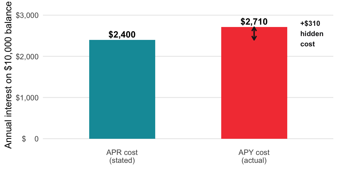
APR (Annual Percentage Rate): The stated annual interest rate, not accounting for compounding.
APY (Annual Percentage Yield): The effective annual rate, including the impact of compounding.
Credit card companies quote APR, but compounding means you actually pay more. Both bars below represent one year’s interest on a $10,000 balance — the taller one is what you really owe.
The formula converts the stated rate into the effective rate by accounting for how many times interest compounds within the year.
Formula: APY = (1 + APR/n)^n − 1
Where n = number of compounding periods per year.
Example: A credit card with a 24% APR compounded daily
APY = (1 + 0.24/365)^365 − 1 = ~27.1%
That 3.1% gap is real money. On a $10,000 balance, it’s an extra $310/year you didn’t realize you were paying.
show/hide
apr_to_apy <- function(apr, periods_per_year = 365) {
  (1 + apr / periods_per_year)^periods_per_year - 1
}

# 24% APR compounded daily
apr_to_apy(apr = 0.24)
#> [1] 0.2711489
show/hide
def apr_to_apy(apr, periods_per_year=365):
    return (1 + apr / periods_per_year) ** periods_per_year - 1

# 24% APR compounded daily
apr_to_apy(apr=0.24)
#> 0.27114889144128895
Minimum Payments
This is the single most important debt calculation you can master. Credit card companies set minimum payments low because the longer you pay, the more they earn.
A $100 minimum payment on a $5,000 credit card balance sounds reasonable — until you see how little of it actually reduces the debt.
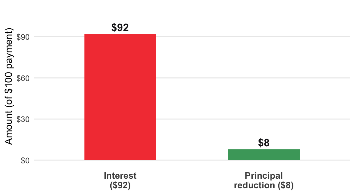
The payoff time formula divides the balance by only the principal slice — the green bar — because that’s the only part that shrinks the debt.
Quick approximation for credit card payoff time:
Months to pay off ≈ Balance ÷ (Monthly Payment − Monthly Interest)
Where: Monthly Interest = Balance × (APR ÷ 12)
Example: $5,000 balance at 22% APR, paying $100/month minimum
Monthly interest: $5,000 × (0.22/12) = ~$92
Effective principal reduction: $100 − $92 = $8/month
Payoff time: $5,000 ÷ $8 = ~625 months (52 years)
That’s not a typo. Minimum payments are designed to keep you in debt for life.
show/hide
months_to_payoff <- function(balance, monthly_payment, apr) {
  monthly_interest    <- balance * (apr / 12)
  principal_reduction <- monthly_payment - monthly_interest
  balance / principal_reduction
}

# $5,000 balance, $100/month, 22% APR
months_to_payoff(balance = 5000, monthly_payment = 100, apr = 0.22)
#> [1] 600
show/hide
def months_to_payoff(balance, monthly_payment, apr):
    monthly_interest    = balance * (apr / 12)
    principal_reduction = monthly_payment - monthly_interest
    return balance / principal_reduction

# $5,000 balance, $100/month, 22% APR
months_to_payoff(balance=5000, monthly_payment=100, apr=0.22)
#> 600.0000000000003
Total Interest Over a Loan’s Life
For any installment loan (car, mortgage, student loan), this is the number that should drive your decisions.
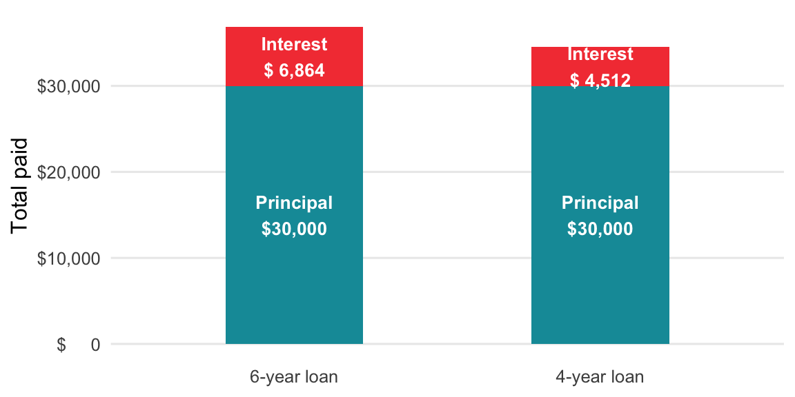
The sticker price is the same $30,000, but the loan term determines how much extra you pay in interest. The chart below stacks the principal and interest layers so the true cost of each term is visible.
Subtract the principal from the total payments and the interest layer is what’s left — that’s the formula.
Formula: Total Interest = (Monthly Payment × Number of Payments) − Loan Principal
Example: $30,000 car loan at 7% for 6 years (~$512/month):
Total paid: $512 × 72 = $36,864
Total interest: $36,864 − $30,000 = $6,864 in interest
Now run the same loan at 4 years instead of 6:
Monthly payment: ~$719
Total paid: $719 × 48 = $34,512
Total interest: $4,512
You save $2,352 by shortening the term: the math behind the 20/4/10 car rule.
show/hide
total_interest <- function(monthly_payment, n_months, principal) {
  (monthly_payment * n_months) - principal
}

# 6-year car loan vs. 4-year, $30,000 principal
total_interest(monthly_payment = 512, n_months = 72, principal = 30000)
#> [1] 6864
total_interest(monthly_payment = 719, n_months = 48, principal = 30000)
#> [1] 4512
show/hide
def total_interest(monthly_payment, n_months, principal):
    return (monthly_payment * n_months) - principal

# 6-year car loan vs. 4-year, $30,000 principal
print(total_interest(monthly_payment=512, n_months=72, principal=30000))
#> 6864
print(total_interest(monthly_payment=719, n_months=48, principal=30000))
#> 4512
Student Loan-to-Income & Standard Payment
The 1× rule from Choosing a Major needs two calculations: the ratio of total debt to expected first-year salary, and the standard 10-year monthly payment that ratio produces.
show/hide
loan_income_ratio <- function(loan_total, expected_salary) {
  loan_total / expected_salary
}

monthly_standard_payment <- function(principal, annual_rate = 0.065, years = 10) {
  r <- annual_rate / 12
  n <- years * 12
  principal * (r * (1 + r)^n) / ((1 + r)^n - 1)
}

# $45,000 in loans, $42,000 expected starting salary
loan_income_ratio(loan_total = 45000, expected_salary = 42000)
#> [1] 1.071429

# standard 10-year monthly payment on that $45,000
monthly_standard_payment(principal = 45000)
#> [1] 510.9659
show/hide
def loan_income_ratio(loan_total, expected_salary):
    return loan_total / expected_salary

def monthly_standard_payment(principal, annual_rate=0.065, years=10):
    r = annual_rate / 12
    n = years * 12
    return principal * (r * (1 + r)**n) / ((1 + r)**n - 1)

# $45,000 in loans, $42,000 expected starting salary
print(loan_income_ratio(loan_total=45000, expected_salary=42000))
#> 1.0714285714285714

# standard 10-year monthly payment on that $45,000
print(monthly_standard_payment(principal=45000))
#> 510.96589749011986
Income-Driven Repayment Monthly Payment
When the 1× rule is out of reach, federal IDR plans cap monthly payments as a percentage of discretionary income, where:
Discretionary income = AGI − (threshold × Federal Poverty Guideline)
The function below takes the AGI, the FPG threshold multiplier (1.5 for IBR/PAYE, 2.25 for SAVE), and the payment rate (0.10 for most plans, 0.05 for SAVE undergraduate loans), and returns the monthly payment.
show/hide
idr_monthly_payment <- function(agi,
                                poverty_guideline = 15650,
                                threshold_pct     = 1.5,
                                payment_rate      = 0.10) {
  discretionary <- max(0, agi - poverty_guideline * threshold_pct)
  round((discretionary * payment_rate) / 12, 2)
}

# IBR: $50,000 AGI, 150% FPG threshold, 10% rate
idr_monthly_payment(agi = 50000)
#> [1] 221.04

# SAVE parameters: 225% FPG threshold, 5% rate (undergraduate loans)
idr_monthly_payment(agi = 50000, threshold_pct = 2.25, payment_rate = 0.05)
#> [1] 61.61
show/hide
def idr_monthly_payment(agi, poverty_guideline=15650,
                        threshold_pct=1.5, payment_rate=0.10):
    discretionary = max(0, agi - poverty_guideline * threshold_pct)
    return round((discretionary * payment_rate) / 12, 2)

# IBR: $50,000 AGI, 150% FPG threshold, 10% rate
print(idr_monthly_payment(agi=50000))
#> 221.04

# SAVE parameters: 225% FPG threshold, 5% rate (undergraduate loans)
print(idr_monthly_payment(agi=50000, threshold_pct=2.25, payment_rate=0.05))
#> 61.61
Debt-to-Income Ratio (DTI)
This is what lenders calculate about you. You should calculate it about yourself.
Lenders look at how much of your gross income is already spoken for by debt. The chart below shows your income divided into what goes to debt and what you actually keep.
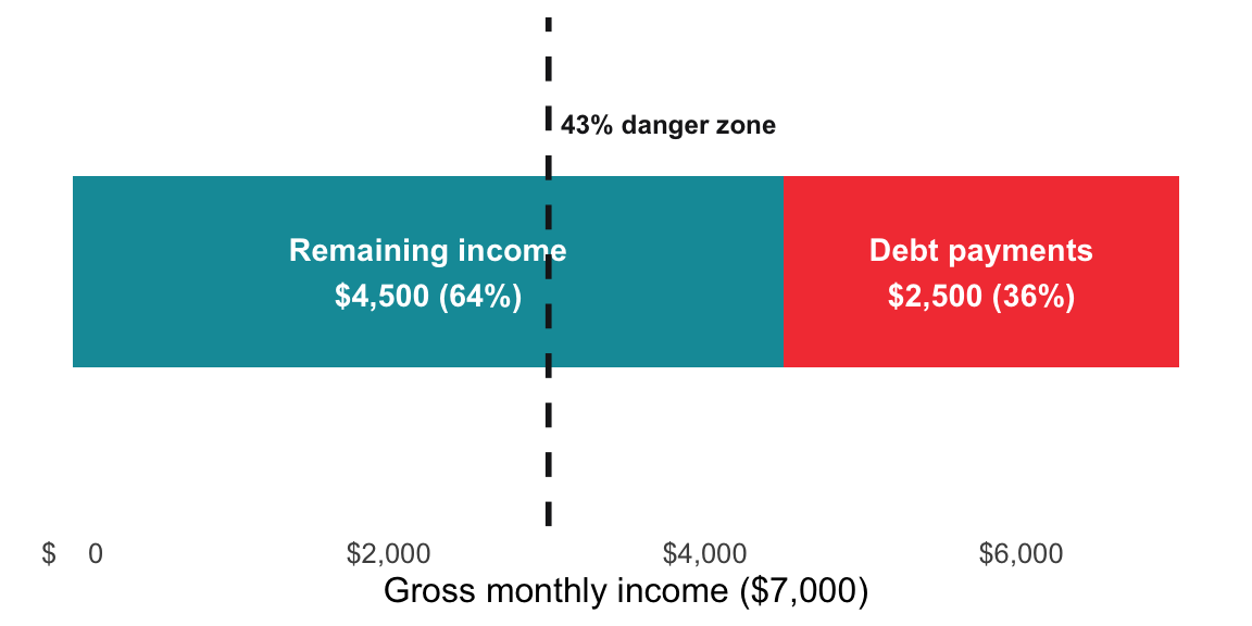
DTI is just the debt slice as a fraction of the whole income bar, expressed as a percentage.
Formula: DTI = (Total Monthly Debt Payments ÷ Gross Monthly Income) × 100
Example:
$2,500 in monthly debt payments on $7,000 gross income → 2,500 ÷ 7,000 = ~36% DTI
Benchmarks:
Below 20%: Healthy
20-35%: Manageable but watch carefully
36-43%: Stretched; lenders get cautious
Above 43%: Danger zone; most mortgage lenders won’t approve you
show/hide
dti_ratio <- function(monthly_debt_payments, gross_monthly_income) {
  (monthly_debt_payments / gross_monthly_income) * 100
}

# $2,500 in debt payments on $7,000 gross income
dti_ratio(monthly_debt_payments = 2500, gross_monthly_income = 7000)
#> [1] 35.71429
show/hide
def dti_ratio(monthly_debt_payments, gross_monthly_income):
    return (monthly_debt_payments / gross_monthly_income) * 100

# $2,500 in debt payments on $7,000 gross income
dti_ratio(monthly_debt_payments=2500, gross_monthly_income=7000)
#> 35.714285714285715
Pay-Off vs. Invest Comparison
This is the math behind every “should I pay extra on my mortgage or invest?” debate.
The math slightly favors investing when the loan rate is below expected returns — but the chart adds what the math alone misses: one bar is certain, the other is a probability.
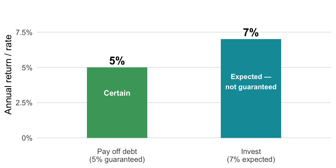
When the investment bar exceeds the debt bar, the math says invest; when the debt bar is higher, pay off — but the certainty premium for debt payoff is worth something the formula can’t capture.
The rule of thumb:
If after-tax loan interest rate > expected after-tax investment return → Pay off the debt If after-tax loan interest rate < expected after-tax investment return → Invest the difference
Example: 5% mortgage vs. expected 7% stock market return (real)
The math favors investing by ~2% per year
But: the loan return is guaranteed, the investment return is not
This is where Housel’s wisdom matters: a guaranteed 5% beats a probable 7% for many people psychologically. Run the math, then add your peace-of-mind premium.
show/hide
payoff_vs_invest <- function(loan_rate, expected_return) {
  if (loan_rate > expected_return) {
    "Pay off the debt"
  } else if (loan_rate < expected_return) {
    "Invest the difference"
  } else {
    "Roughly a wash; do both"
  }
}

# 5% mortgage vs. expected 7% return
payoff_vs_invest(loan_rate = 0.05, expected_return = 0.07)
#> [1] "Invest the difference"
show/hide
def payoff_vs_invest(loan_rate, expected_return):
    if loan_rate > expected_return:
        return "Pay off the debt"
    elif loan_rate < expected_return:
        return "Invest the difference"
    else:
        return "Roughly a wash - do both"

# 5% mortgage vs. expected 7% return
payoff_vs_invest(loan_rate=0.05, expected_return=0.07)
#> 'Invest the difference'
Avalanche vs. Snowball Math
For multiple debts, the choice between methods has a calculable cost.
Both methods attack the same three debts, but in different order. The chart below lays the debts out in each order so the trade-off is visible: avalanche minimizes total interest, snowball builds momentum fastest.
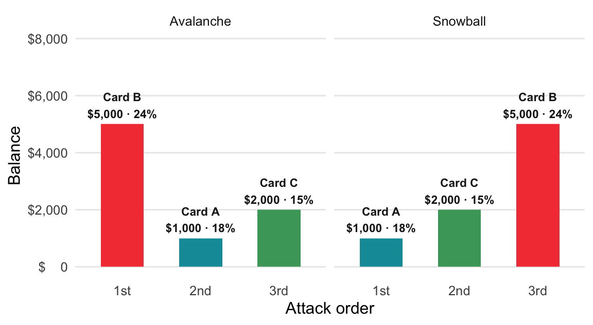
There’s no formula for which order to choose — the code returns the sorted debt list so you can see the order and decide.
Avalanche method: Highest APR first. Mathematically optimal.
Snowball method: Smallest balance first. Psychologically motivating.
- The hidden cost of snowball: To calculate, find total interest paid under each method using a debt payoff calculator. The difference is what you’re “paying” for the psychological win of quick early payoffs.
For most people with moderate debt, the snowball costs $200-$1,000 extra in interest. If that’s the price of actually finishing the journey, it’s often worth it. If you’re disciplined enough for avalanche, take the savings.
These two functions take a list of your debts and return them in the order each method says to attack them.
show/hide
# avalanche: highest APR first
order_avalanche <- function(debts) {
  debts[order(-debts$apr), ]
}

# snowball: smallest balance first
order_snowball <- function(debts) {
  debts[order(debts$balance), ]
}

# your debts, as a small table
debts <- data.frame(
  name    = c("Card A", "Card B", "Card C"),
  balance = c(1000, 5000, 2000),
  apr     = c(0.18, 0.24, 0.15)
)

order_avalanche(debts)
#> # A tibble: 3 × 3
#>   name   balance   apr
#>   <chr>    <dbl> <dbl>
#> 1 Card B    5000  0.24
#> 2 Card A    1000  0.18
#> 3 Card C    2000  0.15
order_snowball(debts)
#> # A tibble: 3 × 3
#>   name   balance   apr
#>   <chr>    <dbl> <dbl>
#> 1 Card A    1000  0.18
#> 2 Card C    2000  0.15
#> 3 Card B    5000  0.24
show/hide
# avalanche: highest APR first
def order_avalanche(debts):
    return sorted(debts, key=lambda d: d["apr"], reverse=True)

# snowball: smallest balance first
def order_snowball(debts):
    return sorted(debts, key=lambda d: d["balance"])

# your debts, as a list of small records
debts = [
    {"name": "Card A", "balance": 1000, "apr": 0.18},
    {"name": "Card B", "balance": 5000, "apr": 0.24},
    {"name": "Card C", "balance": 2000, "apr": 0.15},
]

order_avalanche(debts)
#> [{'name': 'Card B', 'balance': 5000, 'apr': 0.24}, {'name': 'Card A', 'balance': 1000, 'apr': 0.18}, {'name': 'Card C', 'balance': 2000, 'apr': 0.15}]
order_snowball(debts)
#> [{'name': 'Card A', 'balance': 1000, 'apr': 0.18}, {'name': 'Card C', 'balance': 2000, 'apr': 0.15}, {'name': 'Card B', 'balance': 5000, 'apr': 0.24}]
Credit Utilization Ratio
For credit score health, this calculation matters month to month.
Credit scores penalize high utilization — not because the credit bureau is arbitrary, but because using a large fraction of available credit signals financial stress.
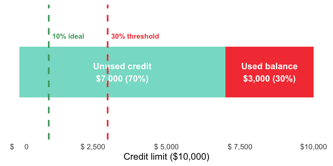
Utilization is just the used slice as a fraction of the total bar, converted to a percentage.
Formula: Utilization = (Current Balance ÷ Credit Limit) × 100
Keep this under 30% on any individual card and across all cards in total. Under 10% is ideal for maximum score impact.
Example: $3,000 balance on $10,000 limit = 30% utilization, right at the threshold.
show/hide
credit_utilization <- function(balance, credit_limit) {
  (balance / credit_limit) * 100
}

# $3,000 balance on a $10,000 limit
credit_utilization(balance = 3000, credit_limit = 10000)
#> [1] 30
show/hide
def credit_utilization(balance, credit_limit):
    return (balance / credit_limit) * 100

# $3,000 balance on a $10,000 limit
credit_utilization(balance=3000, credit_limit=10000)
#> 30.0
4.8 Putting the Math to Work
%%{init: {'theme': 'neutral', 'themeVariables': { 'fontFamily': 'monospace', "fontSize":"16px"}}}%%

flowchart TD
    DebtMath[Debt Math Mastery] --> Decision1[Before Borrowing:<br/>Calculate Total Interest]
    DebtMath --> Decision2[While Paying Off:<br/>Compare APR to Returns]
    DebtMath --> Decision3[Managing Credit:<br/>Monitor DTI & Utilization]

    Decision1 --> Outcome[Intentional<br/>Borrowing Decisions]
    Decision2 --> Outcome
    Decision3 --> Outcome

    Outcome --> Freedom[Financial Freedom]
    style DebtMath fill:#48a56a,color:#F5F2E8,stroke:#1C1C1E,stroke-width:2px
    style Decision1 fill:#0e9aa7,color:#F5F2E8,stroke:#1C1C1E,stroke-width:2px
    style Decision2 fill:#0e9aa7,color:#F5F2E8,stroke:#1C1C1E,stroke-width:2px
    style Decision3 fill:#0e9aa7,color:#F5F2E8,stroke:#1C1C1E,stroke-width:2px
    style Outcome fill:#86ddcd,color:#1C1C1E,stroke:#1C1C1E,stroke-width:2px
    style Freedom fill:#86ddcd,color:#1C1C1E,stroke:#1C1C1E,stroke-width:2px
4.9 Key takeaways
Debt management isn’t about avoiding all debt; it’s about being intentional with it. The right framework:
- Eliminate toxic debt ruthlessly. Credit cards first, always.
- Think in human capital. Student loans are an investment; evaluate the return.
- Resist depreciating debt. Cars financed at high rates are wealth-killers.
You don’t need to be a math genius to do this well, but you do need to be numerically fluent in the calculations above — because lenders absolutely are. The math always tells the truth. Marketing tells you what’s possible. Emotions tell you what feels right. The math tells you what’s actually happening to your money.
As Housel reminds us: the goal isn’t to be debt-free for its own sake. The goal is freedom. And freedom comes from controlling your money before it controls you. As Bogle reminded investors: “The miracle of compounding returns is overwhelmed by the tyranny of compounding costs.” The same principle applies in reverse to debt: compounding interest is wealth-destroying when it’s working against you. Master the math, and you take that weapon out of the lender’s hands.