Beeswarm plots
Description
The beeswarm plot uses points to display the distribution of a continuous variable across the levels of a categorical variable.
The points are grouped by level, and the shape (or swarm) of the distribution is mirrored above and below the quantitative axis (similar to a violin plot).
We can create beeswarm plot using geom_jitter() or the ggbeeswarm package.
Getting set up
PACKAGES:
Install packages.
Code
devtools::install_github("eclarke/ggbeeswarm")
library(ggbeeswarm)
install.packages("palmerpenguins")
library(palmerpenguins)
library(ggplot2)
DATA:

Create peng_beeswarm by grouping penguins by species, then calculating the bill_ratio (bill_length_mm / bill_depth_mm), and then removing any missing values from bill_ratio
Code
peng_beeswarm <- palmerpenguins::penguins |>
    dplyr::group_by(species) |>
    dplyr::mutate(bill_ratio = bill_length_mm / bill_depth_mm) |>
    dplyr::filter(!is.na(bill_ratio)) |>
    dplyr::ungroup()
glimpse(peng_beeswarm)
Rows: 342
Columns: 9
$ species <fct> Adelie, Adelie, Adelie, Adelie, Adelie, Adelie, Adel…
$ island <fct> Torgersen, Torgersen, Torgersen, Torgersen, Torgerse…
$ bill_length_mm <dbl> 39.1, 39.5, 40.3, 36.7, 39.3, 38.9, 39.2, 34.1, 42.0…
$ bill_depth_mm <dbl> 18.7, 17.4, 18.0, 19.3, 20.6, 17.8, 19.6, 18.1, 20.2…
$ flipper_length_mm <int> 181, 186, 195, 193, 190, 181, 195, 193, 190, 186, 18…
$ body_mass_g <int> 3750, 3800, 3250, 3450, 3650, 3625, 4675, 3475, 4250…
$ sex <fct> male, female, female, female, male, female, male, NA…
$ year <int> 2007, 2007, 2007, 2007, 2007, 2007, 2007, 2007, 2007…
$ bill_ratio <dbl> 2.090909, 2.270115, 2.238889, 1.901554, 1.907767, 2.…The grammar
CODE:
Create labels with labs()
Initialize the graph with ggplot() and provide data
Map species to the x axis and color
Map bill_ratio to the y axis
Add the ggbeeswarm::geom_beeswarm() layer (with alpha)
Remove the legend with show.legend = FALSE
Code
labs_beeswarm <- labs(
title = "Adult Foraging Penguins",
subtitle = "Bill Length (mm) / Bill Depth (mm) = Bill Ratio",
x = "Species",
y = "Bill Ratio")
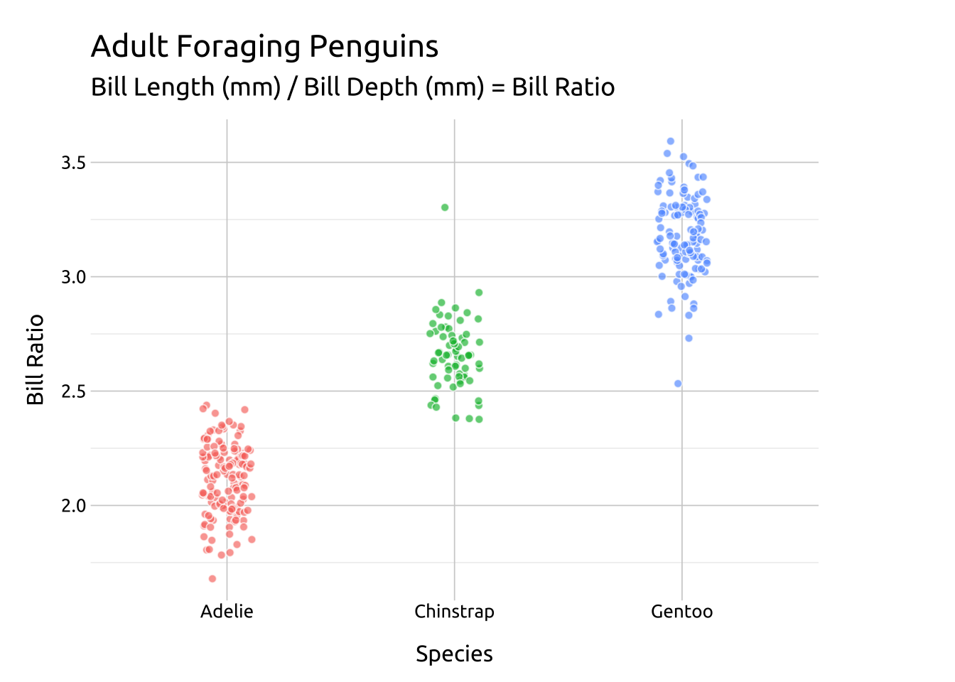
ggp2_beeswarm <- ggplot(data = peng_beeswarm,
aes(x = species,
y = bill_ratio,
color = species)) +
ggbeeswarm::geom_beeswarm(alpha = 2 / 3,
show.legend = FALSE)
ggp2_beeswarm +
labs_beeswarmGRAPH:
Adjust the size/shape of the swarm using method = or the geom_quasirandom() function
More info
Below we cover some additional arguments and methods for beeswarm plots.
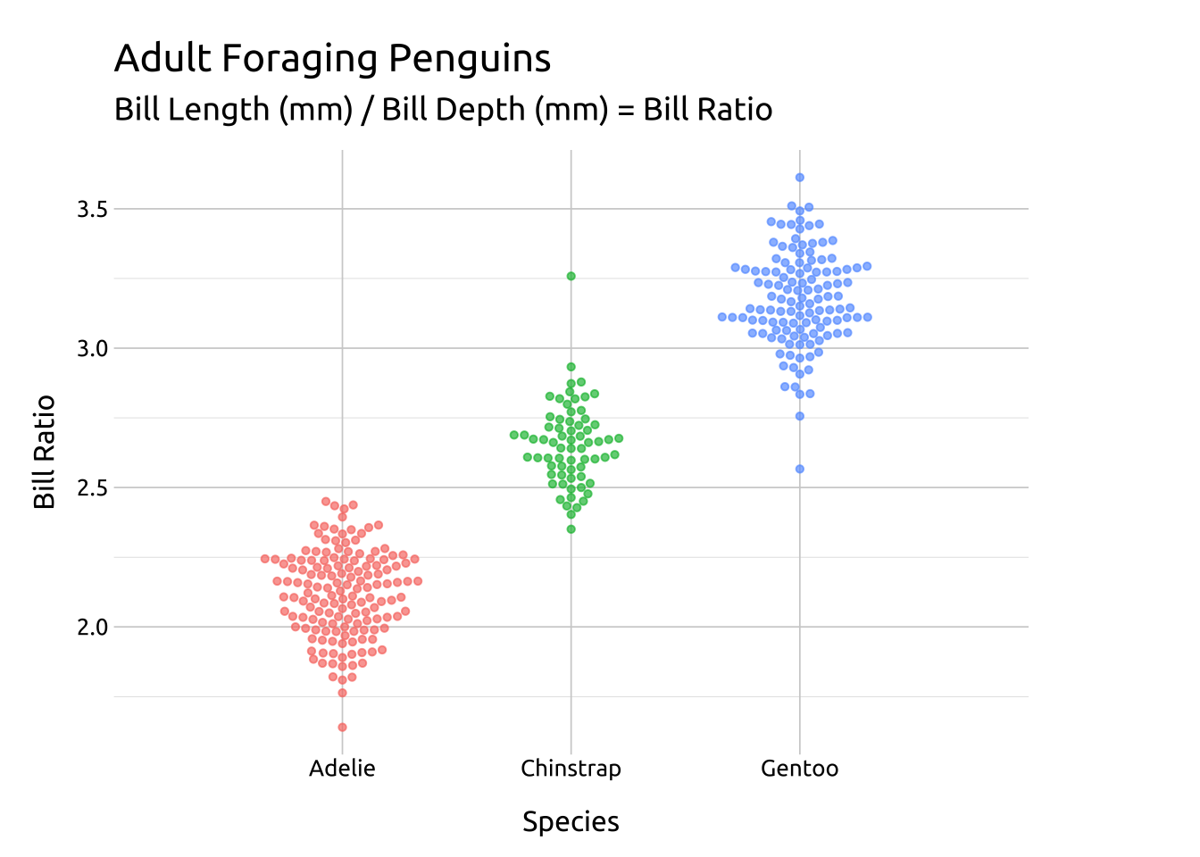
METHOD:
Use method to adjust the shape of the beeswarm (swarm, compactswarm, hex, square, center, or centre)
Set the point shape to 21 to control the fill and color
Code
ggp2_compact_swarm <- ggplot(data = peng_beeswarm,
    mapping = aes(x = species,
                  y = bill_ratio,
                color = species)) +
    ggbeeswarm::geom_beeswarm(
      aes(fill = species),
        method = 'compactswarm',
        dodge.width = 0.5,
        shape = 21,
        color = "#ffffff",
        alpha = 2/3, size = 1.7,
        show.legend = FALSE)
ggp2_compact_swarm +
    # add labels
    labs_beeswarm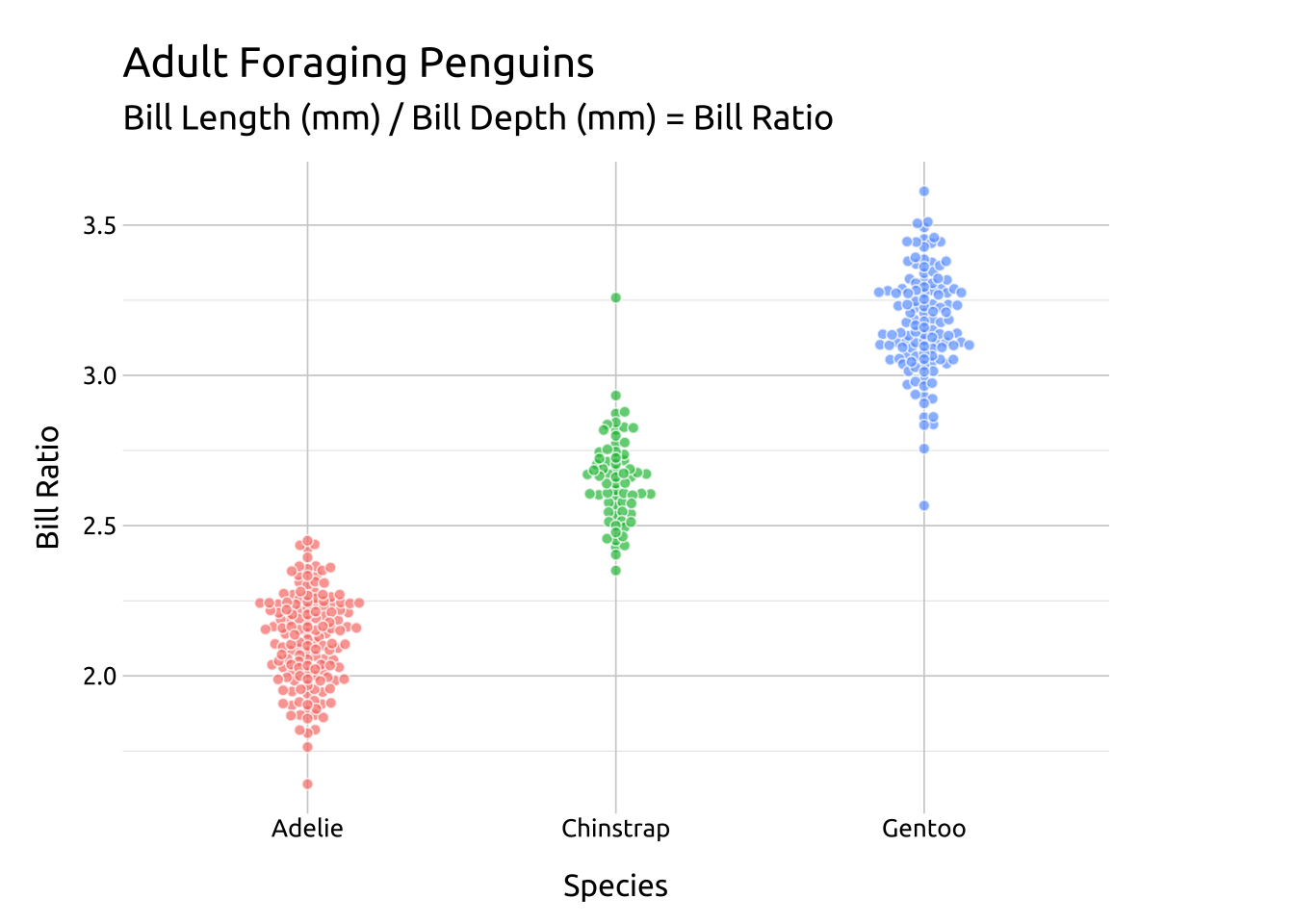
SIDE:
For a beeswarm that falls across the vertical axis, use the side argument.
Code
ggp2_rside_swarm <- ggplot(data = peng_beeswarm,
    mapping = aes(x = species,
                  y = bill_ratio,
                color = species)) +
    ggbeeswarm::geom_beeswarm(
      aes(fill = species),
        side = 1, # right/upwards
        shape = 21,
        color = "#ffffff",
        alpha = 2/3,
        size = 1.7,
        show.legend = FALSE)
ggp2_rside_swarm +
    # add labels
    labs_beeswarm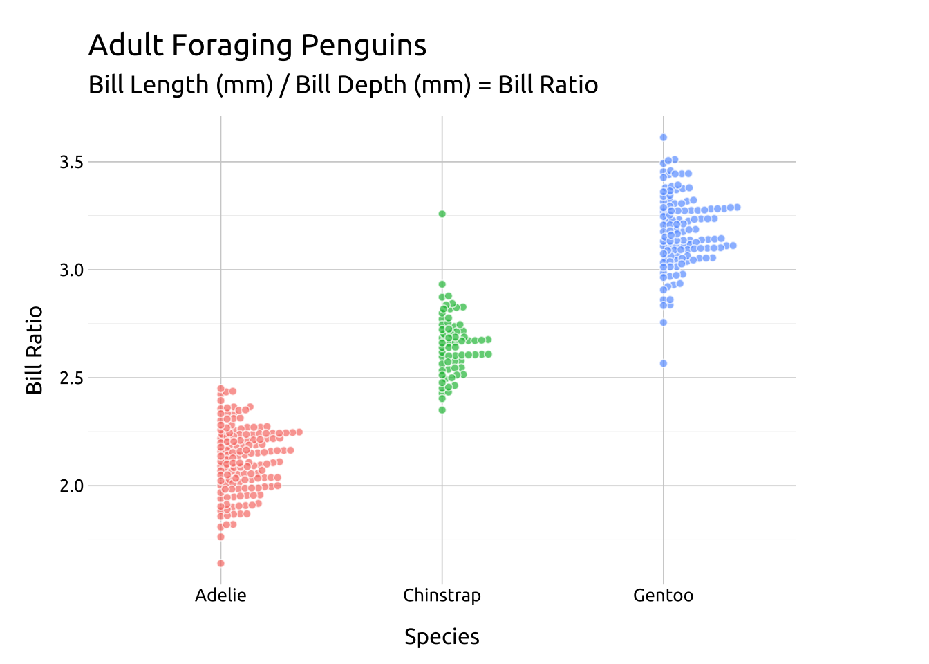
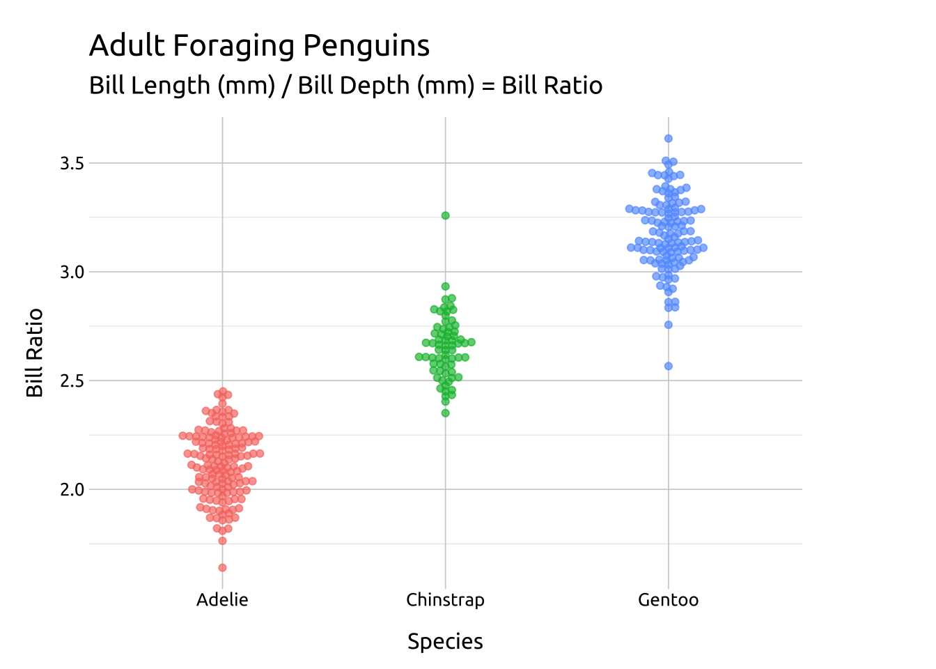
CEX:
The cex argument controls the “scaling for adjusting point spacing”
Code
ggp2_beeswarm_cex <- ggplot(data = peng_beeswarm,
    mapping = aes(x = species,
                  y = bill_ratio,
                color = species)) +
    ggbeeswarm::geom_beeswarm(
      aes(fill = species),
        cex = 1.6,
        shape = 21,
        color = "#ffffff",
        alpha = 2/3,
        size = 1.7,
        show.legend = FALSE)
ggp2_beeswarm_cex +
    # add labels
    labs_beeswarm
JITTER:
We can also create a beeswarm using the geom_jitter() and setting the height and width.
Code
ggp2_jitter_swarm <- ggplot(data = peng_beeswarm,
    mapping = aes(x = species,
        y = bill_ratio,
        color = species)) +
    geom_jitter(
        aes(fill = species),
        height = 0.05,
        width = 0.11,
        shape = 21,
        color = "#ffffff",
        alpha = 2 / 3,
        size = 1.7,
        show.legend = FALSE)
ggp2_jitter_swarm +
    # add labels
    labs_beeswarm