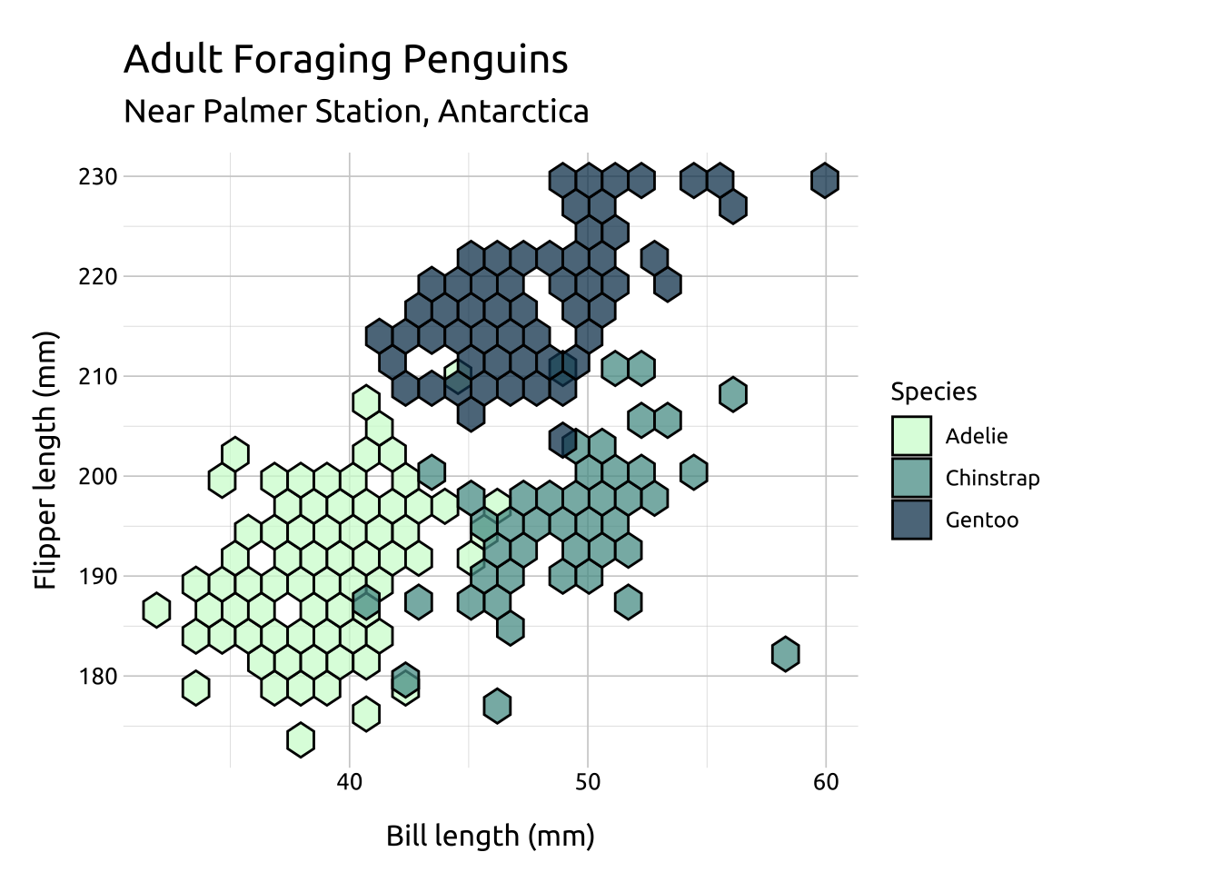
--- title: "Hexagon bins" format: html: toc: true toc-location: right toc-title: Contents code-fold: true out-height: '100%' out-width: '100%' execute: warning: false message: false --- ```{r} #| label: setup #| message: false #| warning: false #| include: false library (tidyverse)library (lubridate)library (scales)library (knitr)library (kableExtra)library (colorblindr)library (downlit)# options ---- options (repos = "https://cloud.r-project.org" ,dplyr.print_min = 6 , dplyr.print_max = 6 , scipen = 9999 )# fonts ---- library (extrafont)library (sysfonts)# import font :: font_import (paths = "assets/Ubuntu/" ,prompt = FALSE )# add font :: font_add (family = "Ubuntu" , regular = "assets/Ubuntu/Ubuntu-Regular.ttf" )# use font :: showtext_auto ()# add theme source ("R/theme_ggp2g.R" )# set theme :: theme_set (theme_ggp2g (base_size = 15 ))install.packages ("palmerpenguins" )``` ## Graph info <br> ```{r} #| label: full_code_display #| eval: true #| echo: false #| warning: false #| message: false #| out-height: '60%' #| out-width: '60%' #| fig-align: right library (palmerpenguins) library (ggplot2)<- palmerpenguins:: penguins |> :: select (flipper_length_mm, bill_depth_mm,|> :: drop_na ()<- labs (title = "Adult Foraging Penguins" , subtitle = "Near Palmer Station, Antarctica" , x = "Bill length (mm)" , y = "Flipper length (mm)" )<- ggplot (data = penguins_hex,aes (x = bill_length_mm, y = flipper_length_mm)) + geom_hex (bins = 15 )+ ``` `r emo::ji("check")` two numeric (continuous) variable## Description ## Getting set up ### Packages ```{r} #| label: pkg_code_hex #| code-fold: show #| eval: true #| echo: true #| warning: false #| message: false #| results: hide install.packages ("palmerpenguins" )library (palmerpenguins)library (ggplot2)``` ### Data  {fig-align="right" width="100%" height="100%"}<!-- {fig-align="right" width="15%" height="15%"} {fig-align="right" width="20%" height="20%"} --> `flipper_length_mm` , `bill_length_mm` , `bill_depth_mm` , `species` , `sex` , and `island` variables from `palmerpenguins::penguins` and drop the missing values. ```{r} #| label: data_code_hex #| eval: true #| echo: true <- palmerpenguins:: penguins |> :: select (flipper_length_mm, bill_depth_mm,|> :: drop_na ()glimpse (penguins_hex)``` ## The grammar ### Code `labs()` `ggplot()` and provide `data` `bill_length_mm` to the `x` and `flipper_length_mm` to the `y` `geom_hex()` layer```{r} #| label: code_graph_hex #| code-fold: show #| eval: false #| echo: true #| warning: false #| message: false #| out-height: '100%' #| out-width: '100%' #| column: page-inset-right #| layout-nrow: 1 <- labs (title = "Adult Foraging Penguins" , subtitle = "Near Palmer Station, Antarctica" , x = "Bill length (mm)" , y = "Flipper length (mm)" )# graph <- ggplot (data = penguins_hex, aes (x = bill_length_mm, y = flipper_length_mm)) + geom_hex ()+ ``` ### Graph ```{r} #| label: create_graph_hex #| eval: true #| echo: false #| warning: false #| message: false #| out-height: '100%' #| out-width: '100%' #| column: page-inset-right #| layout-nrow: 1 <- labs (title = "Adult Foraging Penguins" ,subtitle = "Near Palmer Station, Antarctica" ,x = "Bill length (mm)" ,y = "Flipper length (mm)" )# graph <- ggplot (data = penguins_hex,aes (x = bill_length_mm, y = flipper_length_mm)) + geom_hex ()+ ``` ## More info ### Bins `bins` to `20` and `15` and save these layers as `ggp2_hex_b20` and `ggp2_hex_b15` .```{r} #| label: bins_hex #| eval: true #| echo: true #| warning: false #| message: false #| out-height: '100%' #| out-width: '100%' #| column: page-inset-right #| layout-nrow: 1 <- ggplot (data = penguins_hex,aes (x = bill_length_mm, y = flipper_length_mm)) + geom_hex (bins = 20 )+ <- ggplot (data = penguins_hex,aes (x = bill_length_mm, y = flipper_length_mm)) + geom_hex (bins = 15 )+ ``` ### Scale `scale_color_discrete_sequential()` and setting `aesthetics` to `"fill"` . `alpha` to make them slightly transparent. ```{r} #| label: scales_2d_hex #| eval: true #| echo: true #| warning: false #| message: false #| out-height: '100%' #| out-width: '100%' #| column: page-inset-right #| layout-nrow: 1 <- labs (title = "Adult Foraging Penguins" , subtitle = "Near Palmer Station, Antarctica" , x = "Bill length (mm)" , y = "Flipper length (mm)" ,fill = "Sex" )ggplot (data = penguins_hex, aes (x = bill_length_mm, y = flipper_length_mm)) + geom_hex (aes (fill = sex), bins = 15 , alpha = 3 / 4 ) + scale_color_discrete_sequential (aesthetics = "fill" , rev = FALSE ,palette = "Viridis" ) + ``` `hcl_palettes(type = ` `"sequential")` ### Options `binwidth` allows us to manually adjust the size of the hexagons.`linewidth` is also helpful when using `alpha` for overlapping values. ```{r} #| label: pals_2d_hex #| eval: true #| echo: true #| warning: false #| message: false #| out-height: '100%' #| out-width: '100%' #| column: page-inset-right #| layout-nrow: 1 <- labs (title = "Adult Foraging Penguins" , subtitle = "Near Palmer Station, Antarctica" , x = "Bill length (mm)" , y = "Flipper length (mm)" ,fill = "Species" )ggplot (data = penguins_hex, aes (x = bill_length_mm, y = flipper_length_mm, fill = species)) + geom_hex (binwidth = c (1.1 , 3 ),linewidth = 0.5 , alpha = 3 / 4 ,color = "#000000" ) + scale_color_discrete_sequential (aesthetics = "fill" , palette = "Dark Mint" ) + ``` `bins` (a single number) or `binwidth` (a numeric vector of `c(x, y)` )