Overlapping bar graphs
Desription
Overlapping bar graphs display counts for categorical levels, resulting in bars differentiated by color and ‘stacked’ on top of each other.
In ggplot2, we can build overlapping bar graphs using the fill argument in geom_bar() or geom_col()
Getting set up
PACKAGES:
Install packages.
Code
install.packages("palmerpenguins")
library(palmerpenguins)
library(ggplot2)
DATA:

Remove missing species from penguins and filter the data to only penguins on "Dream" island.
Code
penguins_ovrlp <- filter(penguins,
                      !is.na(species) &
                            island == "Dream")
glimpse(penguins_ovrlp)
Rows: 124
Columns: 8
$ species <fct> Adelie, Adelie, Adelie, Adelie, Adelie, Adelie, Adel…
$ island <fct> Dream, Dream, Dream, Dream, Dream, Dream, Dream, Dre…
$ bill_length_mm <dbl> 39.5, 37.2, 39.5, 40.9, 36.4, 39.2, 38.8, 42.2, 37.6…
$ bill_depth_mm <dbl> 16.7, 18.1, 17.8, 18.9, 17.0, 21.1, 20.0, 18.5, 19.3…
$ flipper_length_mm <int> 178, 178, 188, 184, 195, 196, 190, 180, 181, 184, 18…
$ body_mass_g <int> 3250, 3900, 3300, 3900, 3325, 4150, 3950, 3550, 3300…
$ sex <fct> female, male, female, male, female, male, male, fema…
$ year <int> 2007, 2007, 2007, 2007, 2007, 2007, 2007, 2007, 2007…The grammar
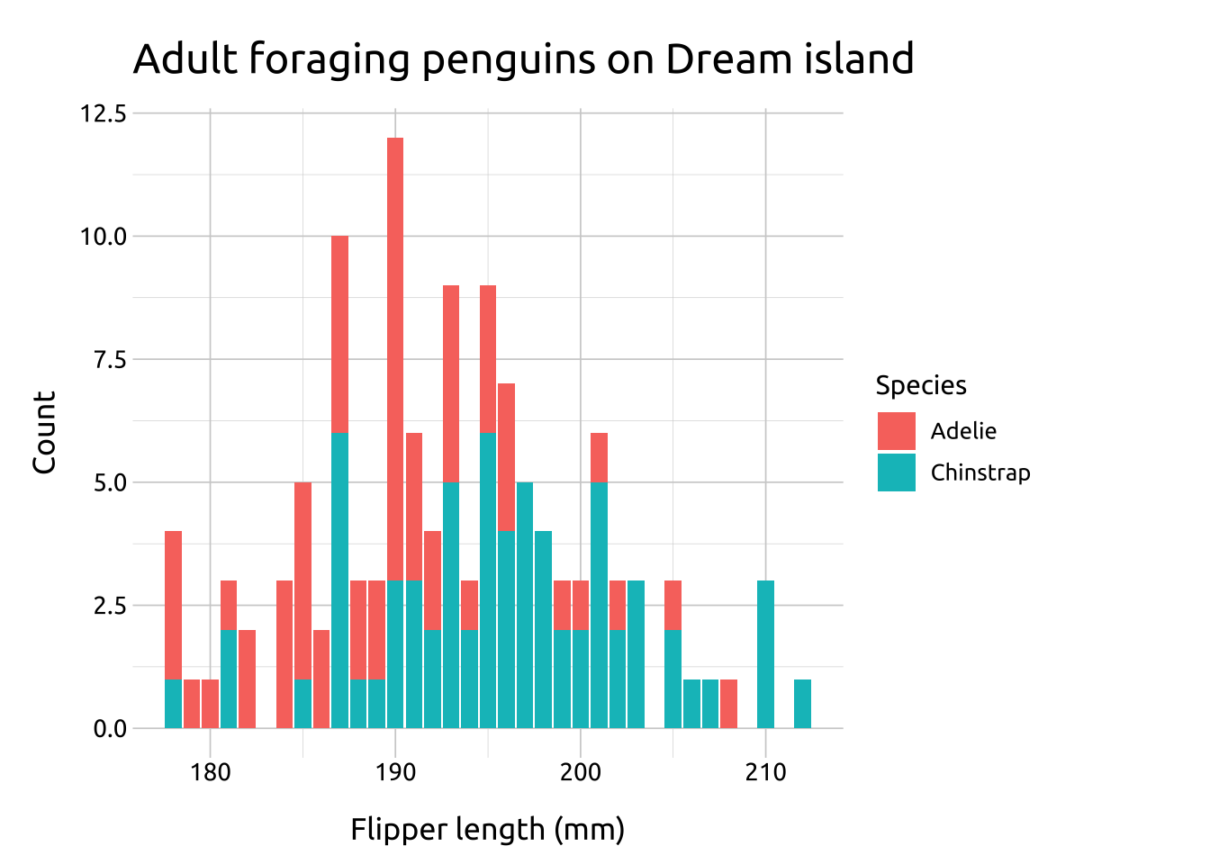
CODE:
Create labels with labs()
Initialize the graph with ggplot() and provide data
Map flipper_length_mm to the x and species to fill
Add the geom_bar() layer
Code
labs_bar_ovrlp <- labs(
  title = "Adult foraging penguins on Dream island",
  x = "Flipper length (mm)",
  y = "Count",
  fill = "Species")
ggp2_bar_ovrlp <- ggplot(data = penguins_ovrlp,
          aes(x = flipper_length_mm, fill = species)) +
                geom_bar()
ggp2_bar_ovrlp +
  labs_bar_ovrlp
GRAPH:

More info
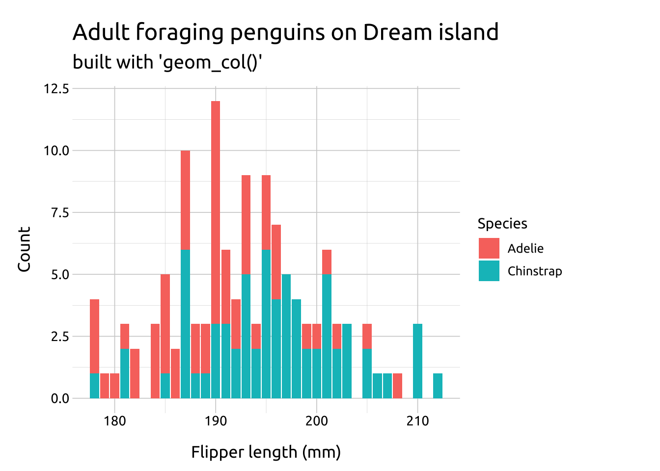
Overlapping bar graphs can also be built with geom_col().
geom_bar() has additional options for arranging overlapping bars. We can set the position argument to "dodge" or "dodge2, depending on how we’d like the data displayed.
geom_col():
To build an overlapping bar graph with geom_col(), we need to create a column with the counts for flipper_length_mm and species in the dataset.
Create the penguins_col data:
Code
penguins_col <- penguins_ovrlp |>
    count(species, flipper_length_mm, name = "Count")
Map the counts to the y axis, flipper_length_mm to the x axis, and species to fill.
Code
labs_col_ovrlp <- labs(
  title = "Adult foraging penguins on Dream island",
  subtitle = "built with 'geom_col()'",
  x = "Flipper length (mm)",
  y = "Count",
  fill = "Species")
ggp2_col_ovrlp <- ggplot(data = penguins_col,
    mapping = aes(y = Count,
        x = flipper_length_mm,
        fill = species)) +
    geom_col()
ggp2_col_ovrlp +
    labs_col_ovrlp
Compare the two graphs below:
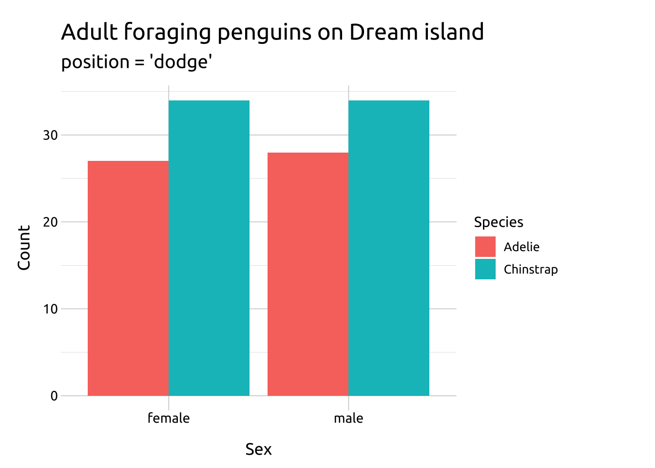
position = "dodge"preserves the vertical position of a geom while adjusting the horizontal positionrequires the grouping variable to be be specified in the global or
geom_ layer
dodge:
Create the penguins_dodge data.
Code
penguins_dodge <- filter(penguins,
                      !is.na(species) &
                        !is.na(sex) &
                            island == "Dream")
glimpse(penguins_dodge)
Rows: 123
Columns: 8
$ species <fct> Adelie, Adelie, Adelie, Adelie, Adelie, Adelie, Adel…
$ island <fct> Dream, Dream, Dream, Dream, Dream, Dream, Dream, Dre…
$ bill_length_mm <dbl> 39.5, 37.2, 39.5, 40.9, 36.4, 39.2, 38.8, 42.2, 37.6…
$ bill_depth_mm <dbl> 16.7, 18.1, 17.8, 18.9, 17.0, 21.1, 20.0, 18.5, 19.3…
$ flipper_length_mm <int> 178, 178, 188, 184, 195, 196, 190, 180, 181, 184, 18…
$ body_mass_g <int> 3250, 3900, 3300, 3900, 3325, 4150, 3950, 3550, 3300…
$ sex <fct> female, male, female, male, female, male, male, fema…
$ year <int> 2007, 2007, 2007, 2007, 2007, 2007, 2007, 2007, 2007…Create labels with labs()
Initialize the graph with ggplot() and provide data
Map species to the x and island to group and fill
Inside the geom_bar() function, set position to "dodge"
Code
labs_bar_dodge <- labs(
  title = "Adult foraging penguins on Dream island",
  subtitle = "position = 'dodge'",
  x = "Sex",
  y = "Count",
  fill = "Species")
ggp2_bar_dodge <- ggplot(data = penguins_dodge,
                    aes(x = sex,
                        group = species,
                        fill = species)) +
                    geom_bar(
                        position = "dodge")
ggp2_bar_dodge +
  labs_bar_dodge
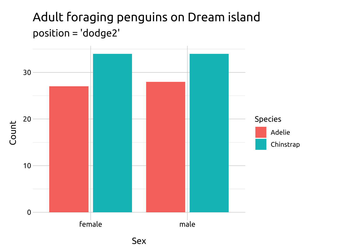
dodge2:
works without a grouping variable in a layer
works with bars and rectangles
useful for arranging graphs with variable widths.
Create labels with labs()
Initialize the graph with ggplot() and provide data
Map species to x and island to fill
Inside geom_bar(), set position to "dodge2"
Code
labs_bar_dodge2 <- labs(
  title = "Adult foraging penguins on Dream island",
  subtitle = "position = 'dodge2'",
  x = "Sex",
  y = "Count",
  fill = "Species")
ggp2_bar_dodge2 <- ggplot(data = penguins_dodge,
                    aes(x = sex,
                        fill = species)) +
                    geom_bar(
                        position = "dodge2")
ggp2_bar_dodge2 +
  labs_bar_dodge2
Compare the two graphs below: