Raincloud plots are a combination of density graph, a box plot, and a beeswarm (or jitter) plot, and are used to compare distributions of quantitative/numerical variables across the levels of a categorical (or discrete) grouping variable.
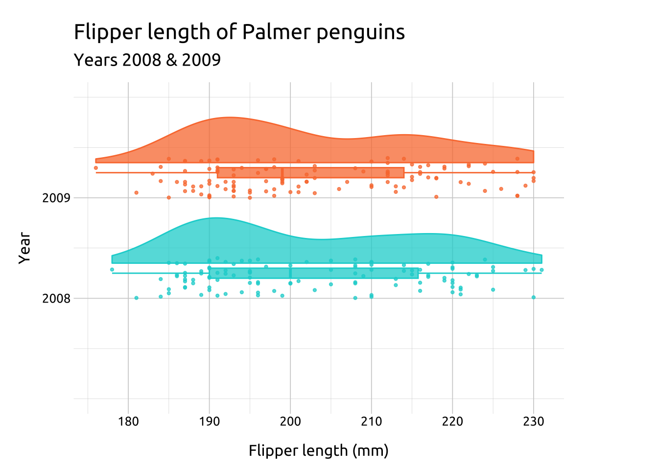
Remove the missing values from year and flipper_length_mm the penguins data. The raincloudplots package has a data_1x1() function we can use to build the dataset for a 1x1 repeated measure graph (peng_1x1).
This function takes two array arguments (array_1 and array_2), which we create with the flipper length (flipper_length_mm) for two levels of year in the peng_raincloud data.
The jit_distance and jit_seed refer to the points in the plot.
Code
# remove missingpeng_raincloud <- palmerpenguins::penguins |>filter(!is.na(year) &!is.na(body_mass_g))# filter flipper length by years 2008 & 2009peng_1x1 <- raincloudplots::data_1x1(array_1 = dplyr::filter(peng_raincloud, year ==2008)$flipper_length_mm,array_2 = dplyr::filter(peng_raincloud, year ==2009)$flipper_length_mm,jit_distance =0.2, # distance between pointsjit_seed =2736) # used in set.seed() glimpse(peng_1x1)
Use the raincloudplots::raincloud_1x1() to build the plot, assigning peng_1x1 to data_1x1
- assign colors and fills
- set the size (of the points) and alpha (for opacity)
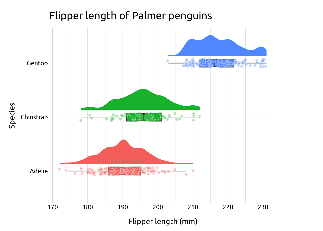
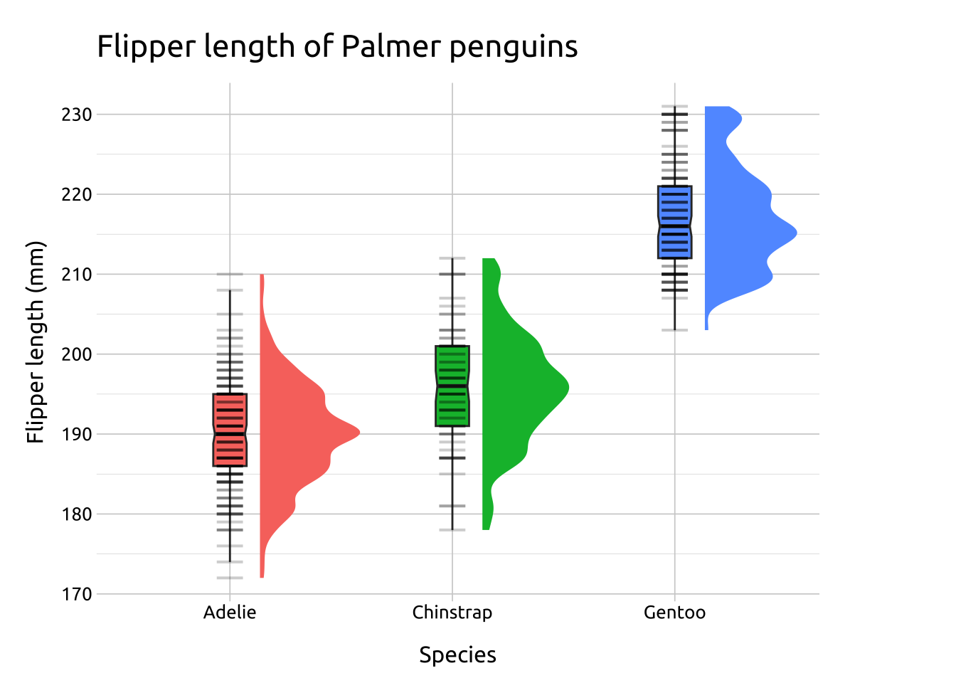
We then add a horizontal density curve with ggdist::stat_halfeye(), mapping species to fill, and adjusting the size and shape of the density curve and shifting it slightly above the box plot.
Code
ggp2_stat_halfeye <- ggp2_box + ggdist::stat_halfeye(aes(fill = species),adjust =0.6, # shape = adjust * density estimator.width =0, # can use probabilities or 0point_colour =NA, # removes the point in centerorientation ="horizontal", # like the box plotheight =0.5, # height of curvejustification =-0.3, # shift vertically above boxshow.legend =FALSE# don't need this ) ggp2_stat_halfeye + labs_raincloud_2
ggplot2::geom_point()
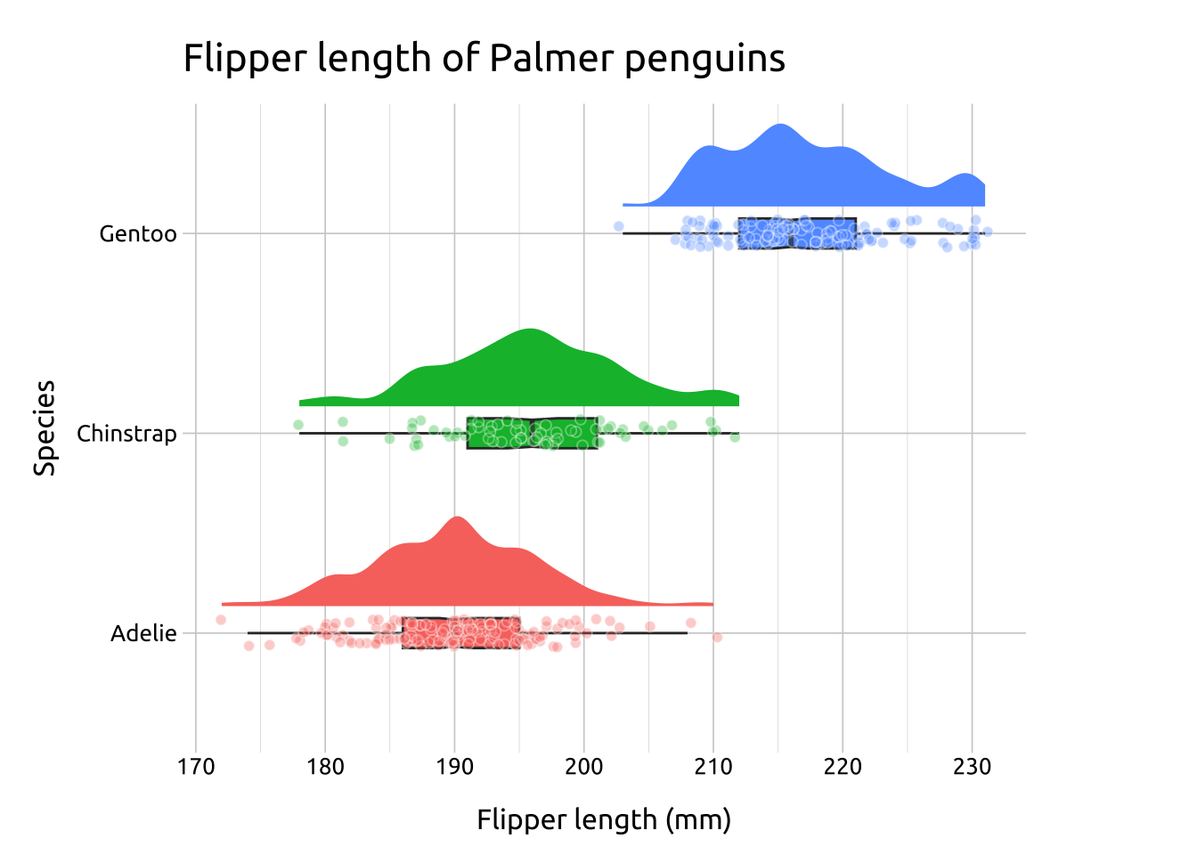
The final layer is a geom_point(), mapping fill to species and setting position to position_jitter(). Additional adjustments to the points include:
Using shape = 21, we can color the outside of the point (white makes it appear to glow).
Manually set the height, which refers to the vertical area for the points
Cédric also covers some alternative methods for plotting the points (I particularly like using bands instead of points when displaying the rainclouds vertically).
We can switch to this layout by applying ggplot2::coord_flip() to the ggp2_stat_halfeye layer, then adding geom_point() with shape set to 95
---title: "Raincloud plots"format: html: toc: true toc-location: right toc-title: Contents code-fold: true out-height: '100%' out-width: '100%'execute: warning: false message: false---```{r}#| label: setup#| message: false#| warning: false#| include: falselibrary(tidyverse)library(lubridate)library(scales)library(knitr)library(kableExtra)library(colorblindr)library(downlit)# options ----options(repos ="https://cloud.r-project.org",dplyr.print_min =6, dplyr.print_max =6, scipen =9999)# fonts ----library(extrafont)library(sysfonts)# import fontextrafont::font_import(paths ="assets/Ubuntu/",prompt =FALSE)# add fontsysfonts::font_add(family ="Ubuntu", regular ="assets/Ubuntu/Ubuntu-Regular.ttf")# use fontshowtext::showtext_auto()# add themesource("R/theme_ggp2g.R")# set themeggplot2::theme_set(theme_ggp2g(base_size =15))install.packages("palmerpenguins")library(palmerpenguins)remotes::install_github('jorvlan/raincloudplots')library(raincloudplots)remotes::install_github('mjskay/ggdist')library(ggdist)```:::: {.callout-note collapse="false" icon=false}## Graph info::: {style="font-size: 1.25em; color: #02577A;"}**Should I use this graph?**:::<br>```{r}#| label: full_code_display#| eval: true#| echo: false#| warning: false#| message: false#| out-height: '60%'#| out-width: '60%'#| fig-align: rightlibrary(raincloudplots)library(ggdist)library(palmerpenguins)library(ggplot2)# remove missingpeng_raincloud <- palmerpenguins::penguins |>filter(!is.na(sex) &!is.na(species))labs_raincloud_2 <- ggplot2::labs(title ="Flipper length of Palmer penguins",x ="Flipper length (mm)",y ="Species")ggplot(peng_raincloud,aes( x = flipper_length_mm, y = species)) +geom_boxplot(aes(fill = species),notch =TRUE, notchwidth =0.9,width = .15, outlier.shape =NA) + ggdist::stat_halfeye(aes(fill = species),adjust =0.6, # shape = adjust * density estimator.width =0, # can use probabilities or 0point_colour =NA, # removes the point in centerorientation ="horizontal", # like the box plotheight =0.5, # height of curvejustification =-0.3) +# shift vertically above boxgeom_point(aes(fill = species),shape =21, color ="#ffffff", alpha =1/3, size =1.8,position =position_jitter(seed =321, height = .07)) +theme(legend.position ="none") + labs_raincloud_2``````{r}#| label: full_code_raincloudplots#| eval: false#| echo: false#| warning: false#| message: false#| out-height: '60%'#| out-width: '60%'#| fig-align: right# filter flipper length by years 2008 & 2009peng_1x1 <- raincloudplots::data_1x1(array_1 = dplyr::filter(peng_raincloud, year ==2008)$flipper_length_mm,array_2 = dplyr::filter(peng_raincloud, year ==2009)$flipper_length_mm,jit_distance =0.2, # distance between pointsjit_seed =2736) # used in set.seed() ggp2_raincloud <-raincloud_1x1(data_1x1 = peng_1x1,colors = (c('#0bd3d3', '#fa7b3c')),fills = (c('#0bd3d3', '#fa7b3c')),size =0.8,alpha =3/4,ort ='h') ggp2_raincloud_x <- ggp2_raincloud +scale_x_continuous(breaks =c(1, 2),labels =c("2008", "2009"),limits =c(0, 3))ggp2_raincloud_x +labs(title ="Flipper length of Palmer penguins",subtitle ="Years 2008 & 2009", x ="Year", y ="Flipper length (mm)")```::: {style="font-size: 1.10em; color: #02577A;"}**This graph requires:**:::::: {style="font-size: 0.90em; color: #043b67;"}`r emo::ji("check")` a categorical variable :::::: {style="font-size: 0.90em; color: #043b67;"}`r emo::ji("check")` a numeric (continuous) variable:::::::## Description Raincloud plots are a combination of density graph, a box plot, and a beeswarm (or jitter) plot, and are used to compare distributions of quantitative/numerical variables across the levels of a categorical (or discrete) grouping variable.We can use the [`raincloudplots` package](https://github.com/jorvlan/raincloudplots) to create raincloud plots, or they can be built using the [`ggdist` package](https://mjskay.github.io/ggdist/) and geoms from `ggplot2`.## Getting set up:::: {.panel-tabset}### Packages::: {style="font-size: 1.15em; color: #1e83c8;"}**PACKAGES:**:::::: {style="font-size: 0.85em;"}Install packages.:::::: {style="font-size: 0.75em;"}```{r}#| label: pkg_code_raincloud#| code-fold: show#| eval: true#| echo: true#| warning: false#| message: false#| results: hideremotes::install_github('jorvlan/raincloudplots')remotes::install_github('mjskay/ggdist')library(raincloudplots)library(ggdist)library(palmerpenguins)library(ggplot2)```:::### Data::: {style="font-size: 1.15em; color: #1e83c8;"}**DATA:**:::::: {style="font-size: 0.85em;"}Remove the missing values from `year` and `flipper_length_mm` the `penguins` data. The `raincloudplots` package has a `data_1x1()` function we can use to build the dataset for a 1x1 repeated measure graph (`peng_1x1`).This function takes two array arguments (`array_1` and `array_2`), which we create with the flipper length (`flipper_length_mm`) for two levels of `year` in the `peng_raincloud` data. The `jit_distance` and `jit_seed` refer to the points in the plot.:::::: {style="font-size: 0.75em;"}```{r}#| label: data_code_raincloud#| eval: true#| echo: true# remove missingpeng_raincloud <- palmerpenguins::penguins |>filter(!is.na(year) &!is.na(body_mass_g))# filter flipper length by years 2008 & 2009peng_1x1 <- raincloudplots::data_1x1(array_1 = dplyr::filter(peng_raincloud, year ==2008)$flipper_length_mm,array_2 = dplyr::filter(peng_raincloud, year ==2009)$flipper_length_mm,jit_distance =0.2, # distance between pointsjit_seed =2736) # used in set.seed() glimpse(peng_1x1)```:::::::## The grammar (`raincloudplots`):::: {.panel-tabset}### Code::: {style="font-size: 1.15em; color: #1e83c8;"}**CODE:**:::::: {style="font-size: 0.85em;"}Create labels with `labs()`Use the `raincloudplots::raincloud_1x1()` to build the plot, assigning `peng_1x1` to `data_1x1` - assign `colors` and `fills` - set the size (of the points) and alpha (for opacity):::::: {style="font-size: 0.75em;"}```{r}#| label: code_graph_raincloud#| code-fold: show#| eval: false#| echo: true #| warning: false#| message: false#| out-height: '100%'#| out-width: '100%'#| column: page-inset-right#| layout-nrow: 1ggp2_raincloud <- raincloudplots::raincloud_1x1(data_1x1 = peng_1x1,colors = (c('#0bd3d3', '#fa7b3c')),fills = (c('#0bd3d3', '#fa7b3c')),size =0.8,alpha =3/4,ort ='h') ggp2_raincloud_x <- ggp2_raincloud + ggplot2::scale_x_continuous(breaks =c(1, 2),labels =c("2008", "2009"),limits =c(0, 3))ggp2_raincloud_x + ggplot2::labs(title ="Flipper length of Palmer penguins",subtitle ="Years 2008 & 2009", x ="Year", y ="Flipper length (mm)")```:::### Graph::: {style="font-size: 1.15em; color: #1e83c8;"}**GRAPH:**:::```{r}#| label: create_graph_raincloud#| eval: true#| echo: false#| warning: false#| message: false#| out-height: '100%'#| out-width: '100%'#| column: page-inset-right#| layout-nrow: 1ggp2_raincloud <- raincloudplots::raincloud_1x1(data_1x1 = peng_1x1,colors = (c('#0bd3d3', '#fa7b3c')),fills = (c('#0bd3d3', '#fa7b3c')),size =0.8,alpha =3/4,ort ='h') ggp2_raincloud_x <- ggp2_raincloud + ggplot2::scale_x_continuous(breaks =c(1, 2),labels =c("2008", "2009"),limits =c(0, 3))ggp2_raincloud_x + ggplot2::labs(title ="Flipper length of Palmer penguins",subtitle ="Years 2008 & 2009", x ="Year", y ="Flipper length (mm)")```::::## More info:::: {.panel-tabset}### Data::: {style="font-size: 1.15em; color: #1e83c8;"}**DATA:**:::::: {.column-margin}{fig-align="right" width="100%" height="100%"}:::::: {style="font-size: 0.85em;"}We'll use the `peng_raincloud` data (with the missing values removed from `species` and `body_mass_g`).:::::: {style="font-size: 0.75em;"}```{r}#| label: data_code_ggdist#| eval: true#| echo: true# remove missingpeng_raincloud <- palmerpenguins::penguins |>filter(!is.na(species) &!is.na(body_mass_g))glimpse(peng_raincloud)```:::### Box-plot::: {style="font-size: 1.15em; color: #1e83c8;"}**`ggplot2::geom_boxplot()`**:::::: {style="font-size: 0.85em;"}Create labels with `labs()`Initialize the graph with `ggplot()` and provide `data`For the first layer, we create a box plot with `geom_boxplot()`, but include notches and remove the outliers. :::::: {style="font-size: 0.75em;"}```{r}#| label: create_graph_raincloud2_box#| eval: true#| echo: true#| warning: false#| message: false#| out-height: '100%'#| out-width: '100%'#| column: page-inset-right#| layout-nrow: 1labs_raincloud_2 <- ggplot2::labs(title ="Flipper length of Palmer penguins",x ="Flipper length (mm)",y ="Species")ggp2_box <-ggplot(peng_raincloud,aes( x = flipper_length_mm, y = species)) +geom_boxplot(aes(fill = species),notch =TRUE, notchwidth =0.9,width =0.15, outlier.shape =NA,show.legend =FALSE)ggp2_box + labs_raincloud_2```:::### Density::: {style="font-size: 1.15em; color: #1e83c8;"}**`ggdist::stat_halfeye()`**:::::: {style="font-size: 0.85em;"}We then add a horizontal density curve with `ggdist::stat_halfeye()`, mapping `species` to `fill`, and adjusting the size and shape of the density curve and shifting it slightly above the box plot.:::::: {style="font-size: 0.75em;"}```{r}#| label: create_graph_raincloud2_halfeye#| eval: true#| echo: true#| warning: false#| message: false#| out-height: '100%'#| out-width: '100%'#| column: page-inset-right#| layout-nrow: 1ggp2_stat_halfeye <- ggp2_box + ggdist::stat_halfeye(aes(fill = species),adjust =0.6, # shape = adjust * density estimator.width =0, # can use probabilities or 0point_colour =NA, # removes the point in centerorientation ="horizontal", # like the box plotheight =0.5, # height of curvejustification =-0.3, # shift vertically above boxshow.legend =FALSE# don't need this ) ggp2_stat_halfeye + labs_raincloud_2```:::### Points::: {style="font-size: 1.15em; color: #1e83c8;"}**`ggplot2::geom_point()`**:::::: {style="font-size: 0.85em;"}The final layer is a `geom_point()`, mapping `fill` to `species` and setting `position` to `position_jitter()`. Additional adjustments to the points include:- Using `shape = 21`, we can `color` the outside of the point (white makes it appear to glow). - Manually set the `height`, which refers to the vertical area for the points :::::: {style="font-size: 0.75em;"}```{r}#| label: create_graph_raincloud2_jitter#| eval: true#| echo: true#| warning: false#| message: false#| out-height: '100%'#| out-width: '100%'#| column: page-inset-right#| layout-nrow: 1ggp2_jitter <- ggp2_stat_halfeye +geom_point(aes(fill = species),position =position_jitter(seed =321, height = .07),shape =21, color ="#ffffff", alpha =1/3, size =1.8,show.legend =FALSE) ggp2_jitter + labs_raincloud_2```:::::::## More examples & resources:::: {.panel-tabset}### Point shape::: {style="font-size: 1.15em; color: #1e83c8;"}**Point shape**:::::: {style="font-size: 0.85em;"}Cédric Scherer covered raincloud plots in [this great write-up](https://www.cedricscherer.com/2021/06/06/visualizing-distributions-with-raincloud-plots-and-how-to-create-them-with-ggplot2/) for [#TidyTuesday](https://github.com/rfordatascience/tidytuesday).Cédric also covers some alternative methods for plotting the points (I particularly like using bands instead of points when displaying the rainclouds vertically).We can switch to this layout by applying `ggplot2::coord_flip()` to the `ggp2_stat_halfeye` layer, then adding `geom_point()` with `shape` set to `95`:::::: {style="font-size: 0.75em;"}```{r}#| label: create_graph_raincloud2_point_lines#| eval: true#| echo: true#| warning: false#| message: false#| out-height: '100%'#| out-width: '100%'#| column: page-inset-right#| layout-nrow: 1ggp2_stat_halfeye + ggplot2::coord_flip() +ggplot2::geom_point(shape =95,size =8,alpha =0.2) +theme(legend.position ="none") + labs_raincloud_2```:::### #TidyTuesday example::: {style="font-size: 1.15em; color: #1e83c8;"}**Polished Graph**:::::: {style="font-size: 0.85em;"}The code to re-create the #TidyTuesday graph is contained in this [gist.](https://gist.github.com/z3tt/8b2a06d05e8fae308abbf027ce357f01){fig-align="center" width="100%" height="100%"}:::### More resources::: {style="font-size: 1.15em; color: #1e83c8;"}**MORE RESOURCES**:::::: {style="font-size: 0.85em;"}1. Raincloud plots: a multi-platform tool for robust data visualization. [1](https://www.ncbi.nlm.nih.gov/pmc/articles/PMC6480976/)2. Shape and point sizes in R. [2](https://r-graphics.org/recipe-scatter-shapes)3. RainCloudPlots package on GitHub. [3](https://github.com/RainCloudPlots/RainCloudPlots):::::::