sap/
├── app.R
└── sap.Rproj
1 directory, 2 files2 Shiny
Note TLDR: Shiny
A basic Shiny project has two files:
An app.R and .Rproj file:
shiny-app/
  ├── app.R
  └── shiny-app.Rproj
A fully developed Shiny project can have the following:
- An
R/folder for additional scripts (i.e., modules, helper & utility functions) that is automatically sourced when the application runs
- The only exception to this is a global.R file, which is run first
A
www/folder for external resources (images, styling, etc.) that is automatically served when the application runsAn optional
DESCRIPTIONfile that controls deployment behaviors (i.e.,DisplayMode)Data files
An optional
README.mdfile for documentation
shiny-app/
  ├── DESCRIPTION
  ├── R/
  │   ├── module.R
  │   ├── helper.R
  │   └── utils.R
  ├── README.md
  ├── app.R
  ├── data.RData
  ├── shiny-app.Rproj
  └── www/
└── shiny.png*Both R/ and www/ are automatically loaded when the app launches.
This chapter briefly reviews programming with Shiny’s reactive model and how it differs from regular R programming. Then, I’ll cover some of the unique behaviors of Shiny app projects (and why you might consider adopting them if you haven’t already).
Shiny basics
Reactivity is the process that lets Shiny apps respond to user actions automatically. When developing Shiny apps, we need to connect inputs, reactivity, and outputs to manage how the app behaves and predict its actions.
Shiny programming is different from regular R programming in a few important ways:
An Event-driven UI: Shiny apps require developers to create a user interface (UI) that helps users navigate the app. The UI registers user actions, such as button clicks or input changes, which trigger updates in the application.1
- Regular R programming often involves executing predefined steps or functions without direct interaction or responses to user events.
A Reactive Server: In Shiny, the app reacts based on how inputs, values, and outputs are connected, which means that when a user makes a change, those changes are automatically shared throughout the app.
- In standard R programming, we write functions to process data and generate outputs like graphs, tables, and model results. This method does not account for reactivity or downstream changes.
Learning reactivity can be challenging when you start, but fortunately, there are excellent tutorials and articles to help you along the way!
2.1 Shiny projects 
Launch app with the shinypak package:
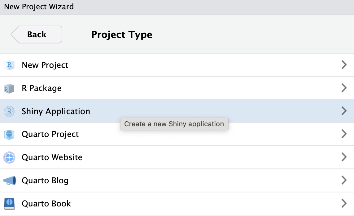
launch('02.1_shiny-app')RStudio’s New Project Wizard ![]() can be used to create a new Shiny application project:
can be used to create a new Shiny application project:
New app projects need a name and location:
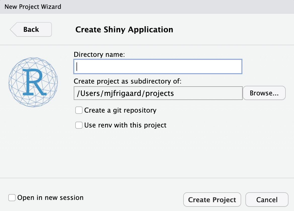
renv2.1.1 Boilerplate app.R
Note that the only items in the new Shiny app project are app.R and the sap.Rproj file.
If you’ve created a new app project in RStudio ![]() , the
, the app.R initially contains a boilerplate application, which we can launch by clicking on the Run App button:

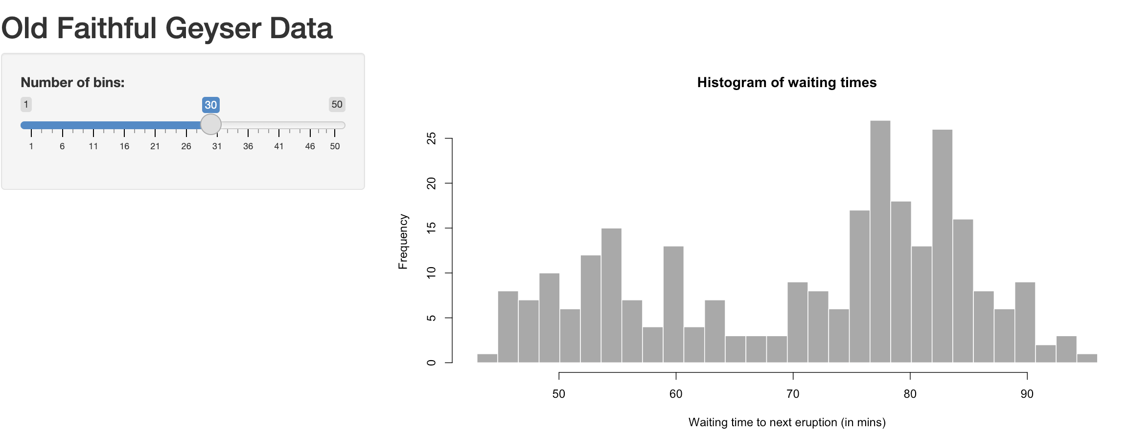
The boilerplate ‘Old Faith Geyser Data’ app is a perfect example of what Shiny can do with a single app.R file, but we’ll want to exchange this code for a more realistic application.
2.2 Movies app
Launch app with the shinypak package:
launch('02.2_movies-app')The next few sections will cover some intermediate/advanced Shiny app features using the Shiny app from the ‘Building Web Applications with Shiny’ course. This app is a great example for the following reasons:
It has multiple input types that are collected in the UI
The graph output can be converted to a utility function
The app loads an external data file when it’s launched
The code is accessible (and comes from a trusted source)
As Shiny applications become more complex, they often grow beyond just one app.R file. Knowing how to store utility functions, data, documentation, and metadata is important to manage this complexity. This preparation helps us successfully organize our Shiny apps into R packages.
2.2.1 app.R
The code below replaces our boilerplate ‘Old Faith Geyser Data’ app in app.R:
show/hide movie review Shiny app
ui <- shiny::fluidPage(
  theme = shinythemes::shinytheme("spacelab"),
  shiny::sidebarLayout(
    shiny::sidebarPanel(
      shiny::selectInput(
        inputId = "y",
        label = "Y-axis:",
        choices = c(
          "IMDB rating" = "imdb_rating",
          "IMDB number of votes" = "imdb_num_votes",
          "Critics Score" = "critics_score",
          "Audience Score" = "audience_score",
          "Runtime" = "runtime"
        ),
        selected = "audience_score"
      ),
      shiny::selectInput(
        inputId = "x",
        label = "X-axis:",
        choices = c(
          "IMDB rating" = "imdb_rating",
          "IMDB number of votes" = "imdb_num_votes",
          "Critics Score" = "critics_score",
          "Audience Score" = "audience_score",
          "Runtime" = "runtime"
        ),
        selected = "critics_score"
      ),
      shiny::selectInput(
        inputId = "z",
        label = "Color by:",
        choices = c(
          "Title Type" = "title_type",
          "Genre" = "genre",
          "MPAA Rating" = "mpaa_rating",
          "Critics Rating" = "critics_rating",
          "Audience Rating" = "audience_rating"
        ),
        selected = "mpaa_rating"
      ),
      shiny::sliderInput(
        inputId = "alpha",
        label = "Alpha:",
        min = 0, max = 1,
        value = 0.4
      ),
      shiny::sliderInput(
        inputId = "size",
        label = "Size:",
        min = 0, max = 5,
        value = 3
      ),
      shiny::textInput(
        inputId = "plot_title",
        label = "Plot title",
        placeholder = "Enter text to be used as plot title"
      ),
      shiny::actionButton(
        inputId = "update_plot_title",
        label = "Update plot title"
      )
    ),
    shiny::mainPanel(
      shiny::br(),
      shiny::p(
        "These data were obtained from",
        shiny::a("IMBD", href = "http://www.imbd.com/"), "and",
        shiny::a("Rotten Tomatoes", href = "https://www.rottentomatoes.com/"), "."
      ),
      shiny::p(
        "The data represent",
        nrow(movies),
        "randomly sampled movies released between 1972 to 2014 in the United States."
      ),
      shiny::plotOutput(outputId = "scatterplot"),
      shiny::hr(),
      shiny::p(shiny::em(
        "The code for this Shiny application comes from",
        shiny::a("Building Web Applications with shiny",
          href = "https://rstudio-education.github.io/shiny-course/"
        )
      ))
    )
  )
)

server <- function(input, output, session) {
  new_plot_title <- shiny::reactive({
    tools::toTitleCase(input$plot_title)
  }) |>
    shiny::bindEvent(input$update_plot_title,
      ignoreNULL = FALSE,
      ignoreInit = FALSE
    )


  output$scatterplot <- shiny::renderPlot({
    scatter_plot(
      df = movies,
      x_var = input$x,
      y_var = input$y,
      col_var = input$z,
      alpha_var = input$alpha,
      size_var = input$size
    ) +
      ggplot2::labs(title = new_plot_title()) +
      ggplot2::theme_minimal() +
      ggplot2::theme(legend.position = "bottom")
  })
}

shiny::shinyApp(ui = ui, server = server)
2.2.2 Utility functions
I’ve converted ggplot2 server code into a scatter_plot() utility function:
show/hide scatter_plot()
scatter_plot <- function(df, x_var, y_var, col_var, alpha_var, size_var) {
    ggplot2::ggplot(data = df,
      ggplot2::aes(x = .data[[x_var]],
          y = .data[[y_var]],
          color = .data[[col_var]])) +
      ggplot2::geom_point(alpha = alpha_var, size = size_var)

}
This function is stored in a new utils.R file:
2.2.3 Data
The movies.RData dataset contains reviews from IMDB and Rotten Tomatoes. You can download these data here. The sap project now contains the following files:
sap/
  ├── app.R
  ├── movies.RData
  ├── sap.Rproj
  └── utils.R

2 directories, 4 files
To run the movies app, we need to load the data and source the utils.R file by adding the code below to the top of the app.R file:
# install ------------------------------------
# install pkgs, then comment or remove below
pkgs <- c("shiny", "shinythemes", "stringr", "ggplot2", "rlang")
install.packages(pkgs, verbose = FALSE)
# packages ------------------------------------
library(shiny)
library(shinythemes)
library(stringr)
library(ggplot2)
library(rlang)
# data -----------------------------------------
load("movies.RData")
# utils ----------------------------------------
source("utils.R")- 1
-
Install
pkgs, then comment or remove below
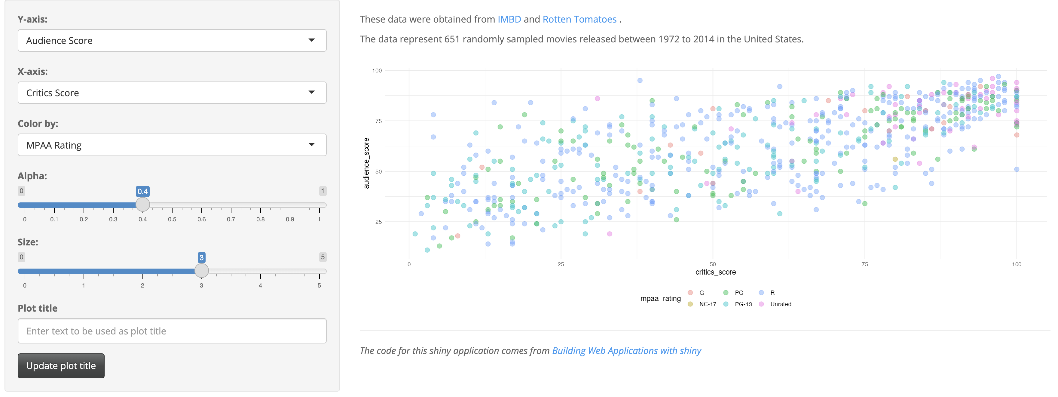
Clicking on Run App displays the movie review app:
2.3 Folders
Now that we have a slightly more complex application in app.R, I’ll add a few project folders we can include in our project that have unique built-in behaviors. These folders will help organize your files and make additional resources available to your app.
Launch app with the shinypak package:
launch('02.3_proj-app')2.3.1 R/
If your Shiny app relies on utility or helper functions outside the app.R file, place this code in an R/ folder. Any .R files in the R/ folder will be automatically sourced when the application is run.
Shiny’s loadSupport() function makes this process possible. We’ll return to this function in a later chapter, because the R/ folder has a similar behavior in R packages.2
2.3.2 www/
When you run a Shiny application, any static files (i.e., resources) under a www/ directory will automatically be made available within the application. This folder stores images, CSS or JavaScript files, and other static resources.
Following the conventional folder structure will also help set you up for success when/if you decide to convert it into an app-package.
2.4 Files
The sections below cover additional files to include in your Shiny app. None of these files are required, but including them will make the transition to package development smoother.
2.4.1 README
Including a README.md file in your root folder is a good practice for any project. Using the standard markdown format (.md) guarantees it can be read from GitHub, too. README.md files should contain relevant documentation for running the application.
2.4.2 DESCRIPTION
DESCRIPTION files play an essential role in R packages, but they are also helpful in Shiny projects if I want to deploy the app in showcase mode.
It’s always a good idea to leave at least one <empty final line> in your DESCRIPTION file.
After adding README.md and a DESCRIPTION file (listing DisplayMode: Showcase), the movies app will display the code and documentation when the app launches.3
2.5 Code
The following two items are considered best practices because they make your app more scalable by converting app.R into functions.
2.5.1 Modules
Shiny modules are a ‘pair of UI and server functions’ designed to compartmentalize input and output IDs into distinct namespaces,
‘…a namespace is to an ID as a directory is to a file…’ -
shiny::NS()help file
Module UI functions usually combine the layout, input, and output functions using tagList(). Module server functions handle the ‘backend’ logic within a Shiny server function. UI and server module functions are connected through an id argument. The UI function creates this id with NS() (namespace), and the server function uses moduleServer() to call it.
2.5.1.1 Inputs
The mod_var_input_ui() function creates a list of inputs (column names and graph aesthetics) in the UI:
show/hide mod_var_input_ui()
mod_var_input_ui <- function(id) {
ns <- shiny::NS(id)
shiny::tagList(
shiny::selectInput(
inputId = ns("y"),
label = "Y-axis:",
choices = c(
"IMDB rating" = "imdb_rating",
"IMDB number of votes" = "imdb_num_votes",
"Critics Score" = "critics_score",
"Audience Score" = "audience_score",
"Runtime" = "runtime"
),
selected = "audience_score"
),
shiny::selectInput(
inputId = ns("x"),
label = "X-axis:",
choices = c(
"IMDB rating" = "imdb_rating",
"IMDB number of votes" = "imdb_num_votes",
"Critics Score" = "critics_score",
"Audience Score" = "audience_score",
"Runtime" = "runtime"
),
selected = "imdb_rating"
),
shiny::selectInput(
inputId = ns("z"),
label = "Color by:",
choices = c(
"Title Type" = "title_type",
"Genre" = "genre",
"MPAA Rating" = "mpaa_rating",
"Critics Rating" = "critics_rating",
"Audience Rating" = "audience_rating"
),
selected = "mpaa_rating"
),
shiny::sliderInput(
inputId = ns("alpha"),
label = "Alpha:",
min = 0, max = 1, step = 0.1,
value = 0.5
),
shiny::sliderInput(
inputId = ns("size"),
label = "Size:",
min = 0, max = 5,
value = 2
),
shiny::textInput(
inputId = ns("plot_title"),
label = "Plot title",
placeholder = "Enter plot title"
)
)
}- 1
-
yaxis numeric variable - 2
-
xaxis numeric variable - 3
-
zaxis categorical variable
- 4
-
alphanumeric value for points
- 5
-
sizenumeric value for size
- 6
-
plot_titletext
%%{init: {'theme': 'neutral', 'themeVariables': { 'fontFamily': 'monospace',"fontSize":"16px"}}}%%
flowchart TD
    User(["User"])
    subgraph mod_var_input_server["<strong>mod_var_input_server()</strong>"]
        XServer[\"input$x"\]
        YServer[\"input$y"\]
        ZServer[\"input$z"\]
        AlphaServer[\"input$alpha"\]
        SizeServer[\"input$size"\]
        TitleServer[\"input$plot_title"\]
    end
    subgraph mod_var_input_ui["<strong>mod_var_input_ui()</strong>"]
        XUI[/"X-axis"/]
        YUI[/"Y-axis"/]
        ZUI[/"Color by"/]
        AlphaUI[/"Alpha"/]
        SizeUI[/"Size"/]
        TitleUI[/"Plot title"/]
    end
    User --> |"<em>Selects...</em>"|mod_var_input_ui
    mod_var_input_ui -->|"<em>Collects...</em>"| mod_var_input_server
    mod_var_input_server --> |"<em>Returns...</em>"|Return(["Reactive<br>list"])
mod_var_input_server() returns these values in a reactive list:
show/hide mod_var_input_server()
mod_var_input_server <- function(id) {
shiny::moduleServer(id, function(input, output, session) {
return(
reactive({
list(
"y" = input$y,
"x" = input$x,
"z" = input$z,
"alpha" = input$alpha,
"size" = input$size,
"plot_title" = input$plot_title
)
})
)
})
}- 1
-
yaxis numeric variable - 2
-
xaxis numeric variable - 3
-
zaxis categorical variable
- 4
-
alphanumeric value for points
- 5
-
sizenumeric value for size
- 6
-
plot_titletext
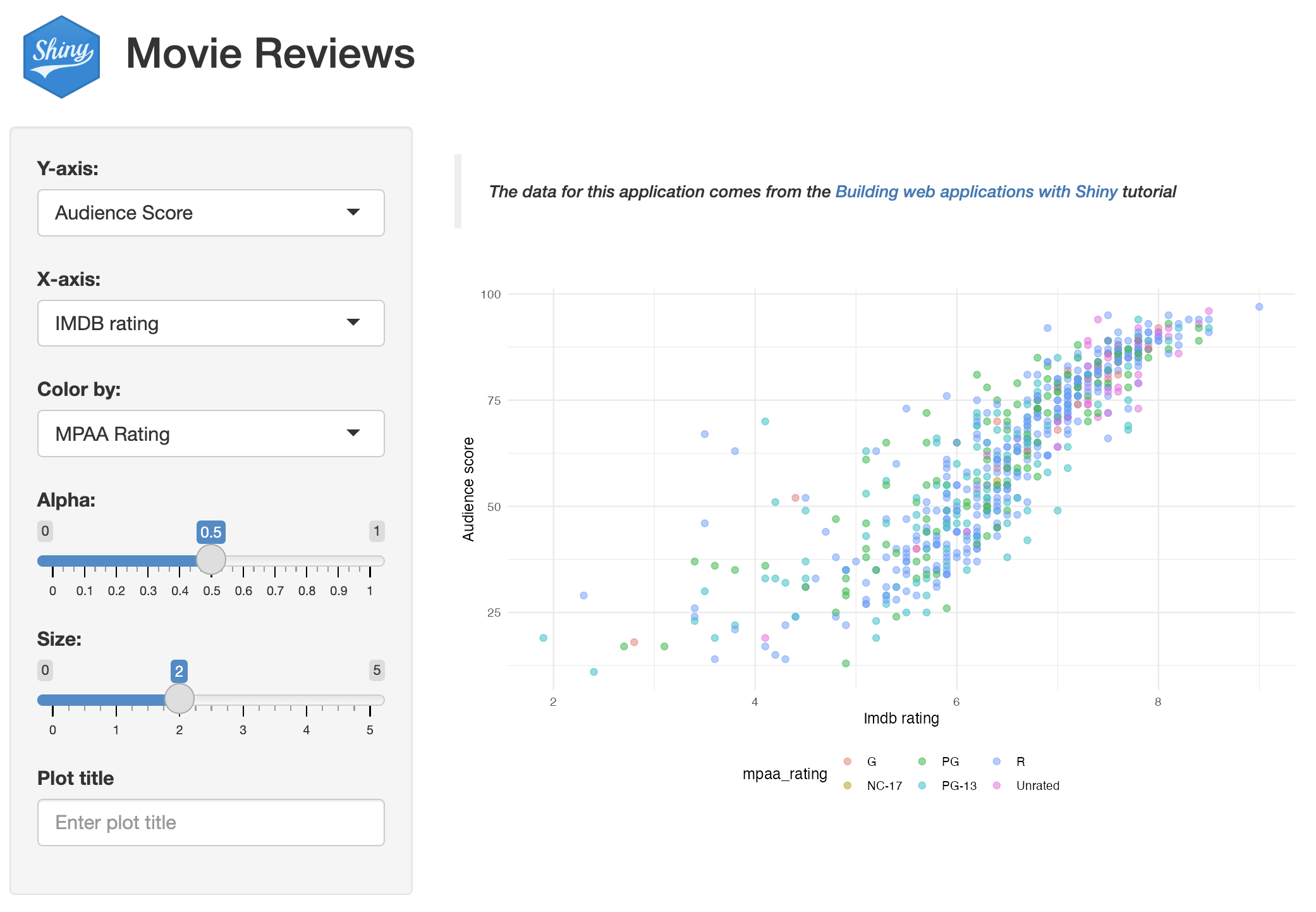
2.5.1.2 Display
mod_scatter_display_ui() creates a dedicated namespace for the plot output (along with some help text):
show/hide mod_scatter_display_ui()
mod_scatter_display_ui <- function(id) {
ns <- shiny::NS(id)
shiny::tagList(
shiny::tags$br(),
shiny::tags$blockquote(
shiny::tags$em(
shiny::tags$h6("The data for this application comes from the ",
shiny::tags$a("Building web applications with Shiny",
href = "https://rstudio-education.github.io/shiny-course/"),
"tutorial"))
),
shiny::plotOutput(outputId = ns("scatterplot"))
)
}- 1
-
Namespaced module
idfor plot in UI
mod_scatter_display_server() loads the movies data and collects the returned reactive list from variable input module as var_inputs.
%%{init: {'theme': 'neutral', 'themeVariables': { 'fontFamily': 'monospace', "fontSize":"16px"}}}%%
flowchart TD
    User(["User"])
    mod_var_input_ui["<strong>mod_var_input_ui()</strong>"]
    mod_scatter_display_ui["<strong>mod_scatter_display_ui</strong>"]

    subgraph mod_scatter_display_server["<strong>mod_scatter_display_server()</strong>"]
        var_inputs[\"var_inputs()"\]
        inputs[\"inputs()"\]
        scatter_plot("scatter_plot()")
    end

    subgraph mod_var_input_server["<strong>mod_var_input_server()</strong>"]
        Reactives[/"input$x<br>input$y<br>input$z<br>input$alpha<br>input$size"/]
        Title[/"input$plot_title"\]
    end

    User --> |"<em>Selects inputs...</em>"|mod_var_input_ui
    mod_var_input_ui --> |"<em>Collects inputs..</em>"|mod_var_input_server
    Reactives -->|"<em>Returns inputs...</em>"|selected_vars
    Title -.-> |"<em>Optional input...</em>"|selected_vars
    selected_vars[/"selected inputs"/] -->|"<em>Input argument for...</em>"|mod_scatter_display_server
    var_inputs --> inputs --> scatter_plot
    scatter_plot -->|"<em>Renders plot...</em>"|mod_scatter_display_ui
    mod_scatter_display_ui -->|"<em>Displays output...</em>"|Display(["Graph"])

    style mod_scatter_display_ui stroke-width:2px,rx:3,ry:3
    style mod_scatter_display_server stroke-width:2px,rx:3,ry:3
    style mod_var_input_ui stroke-width:2px,rx:3,ry:3
    style mod_var_input_server stroke-width:2px,rx:3,ry:3
    style scatter_plot stroke-width:2px,rx:10,ry:10
    style Reactives font-size:15px,stroke-width:1px,rx:5,ry:5
    style Title font-size:15px,stroke-width:1px,rx:5,ry:5
var_inputs() is used to build the inputs() reactive, which is passed to the scatter_plot() utility function. scatter_plot() creates the graph, adds the plot_title() (if necessary) and theme:
show/hide mod_scatter_display_server()
mod_scatter_display_server <- function(id, var_inputs) {
shiny::moduleServer(id, function(input, output, session) {
load("movies.RData")
inputs <- shiny::reactive({
plot_title <- tools::toTitleCase(var_inputs()$plot_title)
list(
x = var_inputs()$x,
y = var_inputs()$y,
z = var_inputs()$z,
alpha = var_inputs()$alpha,
size = var_inputs()$size,
plot_title = plot_title
)
})
output$scatterplot <- shiny::renderPlot({
plot <- scatter_plot(
df = movies,
x_var = inputs()$x,
y_var = inputs()$y,
col_var = inputs()$z,
alpha_var = inputs()$alpha,
size_var = inputs()$size
)
plot +
ggplot2::labs(
title = inputs()$plot_title,
x = stringr::str_replace_all(
tools::toTitleCase(
inputs()$x),
"_", " "),
y = stringr::str_replace_all(
tools::toTitleCase(
inputs()$y),
"_", " ")
) +
ggplot2::theme_minimal() +
ggplot2::theme(legend.position = "bottom")
})
})
}- 1
-
loading the
moviesdata - 2
-
assembling the returned values from
mod_var_input_server(), and creating theinput()reactive - 3
-
scatter_plot()utility function creates theplotobject - 4
-
adds the
plot_title() - 5
-
add
themeto layers
Both UI and server module functions are combined into a single .R file, and all modules are placed in the R/ folder so they are sourced when the application is run.
R/
 ├── mod_scatter_display.R
 ├── mod_var_input.R
 └── utils.R
2.5.2 Standalone app function
Instead of using shiny::shinyApp() (or the Run App icon), we’ll want a custom standalone app function to launch our application. This give us more flexibility and control with our modules (and makes debugging easier).
show/hide launch_app()
launch_app <- function() {
shiny::shinyApp(
ui = shiny::fluidPage(
shiny::titlePanel(
shiny::div(
shiny::img(
src = "shiny.png",
height = 60,
width = 55,
style = "margin:10px 10px"
),
"Movies Reviews"
)
),
shiny::sidebarLayout(
shiny::sidebarPanel(
mod_var_input_ui("vars")
),
shiny::mainPanel(
mod_scatter_display_ui("plot")
)
)
),
server = function(input, output, session) {
selected_vars <- mod_var_input_server("vars")
mod_scatter_display_server("plot", var_inputs = selected_vars)
}
)
}- 1
- Variable input UI module
- 2
- Graph display UI module
- 3
- Variable input server module
- 4
- Graph display server module
The id arguments ("vars" and "plot") connect the UI functions to their server counterparts, and the output from mod_var_input_server() is the var_inputs argument in mod_scatter_display_server().
%%{init: {'theme': 'neutral', 'themeVariables': { 'fontFamily': 'monospace', "fontSize":"13px"}}}%%
flowchart LR
    subgraph Launch["<code>launch_app()</code>"]
        subgraph VarNS["Variable (<code>vars</code>) Namespace"]
            VarInpuUI["UI Module:<br><code>mod_var_input_ui()</code>"]
            VarInpuServer["Server Module:<br><code>mod_var_input_server()</code>"]
            VarInpuUI <--> VarInpuServer
        end
        subgraph GraphNS["Graph (<code>plot</code>) Namespace"]
        DisplayUI["UI Module:<br><code>mod_scatter_display_ui()</code>"]
        DisplayServer["Server Module:<br><code>mod_scatter_display_server()</code>"]
        PlotUtil["Utility Function:<br><code>scatter_plot()</code>"]
        VarInpuServer <-->|"selected_vars"|DisplayServer
        DisplayServer <-.-> PlotUtil <--> DisplayUI
        end
    end

    VarNS <==>|"Communicates<br>across namespaces"| GraphNS
To launch our app, we place the call to shinyApp() in a launch_app() function in app.R. Both module functions are combined in the ui and server arguments of shinyApp().
show/hide launch_app() in app.R
# install ------------------------------------
# after installing, comment this out
pkgs <- c("shiny", "shinythemes", "stringr", "ggplot2", "rlang")
install.packages(pkgs, verbose = FALSE)
# packages ------------------------------------
library(shiny)
library(shinythemes)
library(stringr)
library(ggplot2)
library(rlang)
launch_app <- function() {
shiny::shinyApp(
ui = shiny::fluidPage(
shiny::titlePanel(
shiny::div(
shiny::img(
src = "shiny.png",
height = 60,
width = 55,
style = "margin:10px 10px"
),
"Movies Reviews"
)
),
shiny::sidebarLayout(
shiny::sidebarPanel(
mod_var_input_ui("vars")
),
shiny::mainPanel(
mod_scatter_display_ui("plot")
)
)
),
server = function(input, output, session) {
selected_vars <- mod_var_input_server("vars")
mod_scatter_display_server("plot", var_inputs = selected_vars)
}
)
}
launch_app()- 1
- Header (comment this out after the packages are installed)
- 2
-
Load packages
- 3
- Variable input UI module
- 4
- Graph display UI module
- 5
- Variable input server module
- 6
- Graph display server module
Now, I can run the app with launch_app().
The deployed files of sap are below:
sap/ # 02.3_proj-app branch
├── DESCRIPTION
├── R/
│   ├── mod_scatter_display.R
│   ├── mod_var_input.R
│   └── utils.R
├── README.md
├── app.R
├── movies.RData
├── sap.Rproj
├── rsconnect/
│   └── shinyapps.io/
│       └── user/
│           └── sap.dcf
└── www/
    └── shiny.png

6 directories, 10 files
The rsconnect/ folder has been removed from the 02.3_proj-app branch.
2.6 Additional features
Below are two additional ‘optional’ features that can be included with your Shiny application. I consider these ‘optional’ because they’re use depends on the specific needs and environment for each application.
2.6.1 Globals
Placing a global.R file in your root folder (or in the R/ directory) causes this file to be sourced only once when the Shiny app launches, rather than each time a new user connects to the app. global.R is commonly used for initializing variables, loading libraries, loading large data sets and/or performing initial calculations.
global.R can be used to maintain efficiency and consistency across application sessions.
2.6.2 Project dependencies (renv)
If you use renv to keep track of project-level dependencies, regularly run renv::status() and renv::snapshot() to keep the lockfile updated.
2.7 Recap
This chapter has covered some differences between developing Shiny apps and regular R programming, creating new Shiny projects in Posit Workbench, and some practices to adopt that can make the transition to app-packages a little easier. The code used in this chapter is stored in the sap repository.
In the next chapter, I’ll cover what makes a package a package, and some do’s and don’ts when converting a developed Shiny application into an R package.
Shiny apps require developers to design and develop a user interface (UI). User experience (UX) design is an entirely separate field, but as Shiny developers, we need to know enough to allow users to interact with and navigate our apps.↩︎
Shiny introduced these features in version 1.3.2.9001, and you can read more about them in the section titled, ‘The
R/directory’ in App formats and launching apps↩︎