33  Alluvial charts

This graph is largely complete and just needs final proof reading.

This graph requires:

✅ multiple categorical variables

✅ a date or time variable

33.1 Description

An alluvial graph displays the changes in composition or flow over time or across multiple categories.

We can build alluvial charts in ggplot2 with the ggalluvial package:.

See also: parallel sets

33.2 Set up

PACKAGES:

Install packages.

# pak::pak("corybrunson/ggalluvial")
library(ggalluvial)
install.packages("palmerpenguins")
library(palmerpenguins) 
library(ggplot2)

DATA:

Artwork by allison horst

Below we create a wide example of the penguins data (as peng_wide).

peng_wide <- penguins |> 
  tidyr::drop_na() |> 
  dplyr::count(year, island, sex, species) |> 
  dplyr::mutate(year = factor(year)) |> 
  dplyr::rename(freq = n)
dplyr::glimpse(peng_wide)
#> Rows: 30
#> Columns: 5
#> $ year    <fct> 2007, 2007, 2007, 2007, 2007, 20…
#> $ island  <fct> Biscoe, Biscoe, Biscoe, Biscoe, …
#> $ sex     <fct> female, female, male, male, fema…
#> $ species <fct> Adelie, Gentoo, Adelie, Gentoo, …
#> $ freq    <int> 5, 16, 5, 17, 9, 13, 10, 13, 8, …

33.3 Grammar

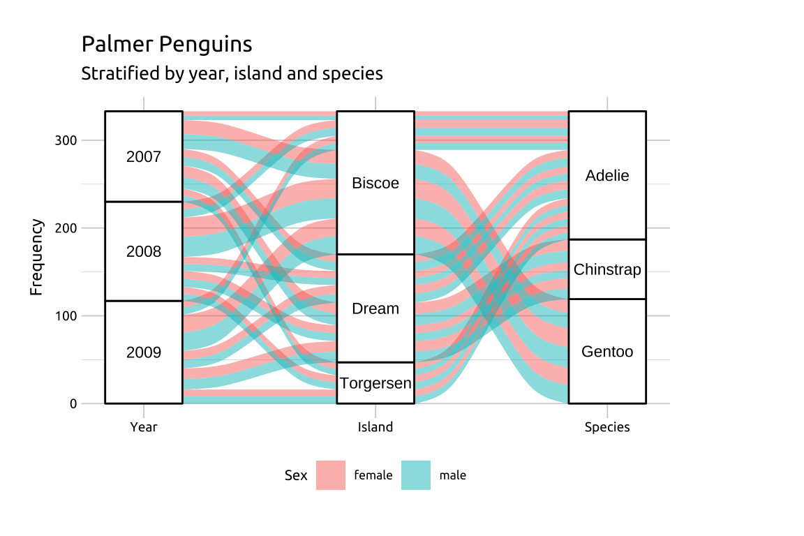
CODE:

• Create labels with labs() (with ggtitle(), ylab(), and labs())

• Add scale_x_discrete() with the limits set to "Year", "Island" and "Species", and expand to 0.1 and 0.07

• Add geom_alluvium() with fill set to the sex variable and geom_stratum()

• Add geom_text(), with stat set to stratum and label set to after_stat(stratum) (inside aes())

labs_alluvial <- ggtitle(label = "Palmer Penguins", 
    subtitle = "Stratified by year, island and species")
labs_alluvial_y <- ylab("Frequency") 
labs_alluvial_fill <- labs(fill = "Sex")

ggp2_alluvial_w <- ggplot(data = peng_wide,
  aes(axis1 = year, axis2 = island,
      axis3 = species, y = freq)) +
  scale_x_discrete(
    limits = c("Year", "Island", "Species"),
    expand = c(0.1, 0.07)) +
  geom_alluvium(aes(fill = sex)) +
  geom_stratum() +
  geom_text(stat = "stratum", 
    aes(label = after_stat(stratum)),
      size = 3)

ggp2_alluvial_w + 
  theme(legend.position = "bottom")
  labs_alluvial + 
  labs_alluvial_y + 
  labs_alluvial_fill

GRAPH:

The ggalluvial functions can handle wide or long data.

33.4 More info

The ggalluvial package can also help reshape data with the to_lodes_form() function.

33.4.1 to_lodes_form()

Below we create peng_lodes from the penguins dataset using the to_lodes_form() from the ggalluvial package.

peng_lodes <- penguins |> 
  dplyr::select(Year = year, Island = island, 
         Species = species, Sex = sex) |> 
  tidyr::drop_na() |> 
  dplyr::count(Year, Island, Species, Sex) |> 
  dplyr::mutate(Year = factor(Year)) |> 
  dplyr::rename(Freqency = n) |> 
  ggalluvial::to_lodes_form(key = "Measure", axes = 1:3) 
glimpse(peng_lodes)
#> Rows: 90
#> Columns: 5
#> $ Sex      <fct> female, male, female, male, fem…
#> $ Freqency <int> 5, 5, 16, 17, 9, 10, 13, 13, 8,…
#> $ alluvium <int> 1, 2, 3, 4, 5, 6, 7, 8, 9, 10, …
#> $ Measure  <fct> Year, Year, Year, Year, Year, Y…
#> $ stratum  <fct> 2007, 2007, 2007, 2007, 2007, 2…

Create labels with labs()

• Map Measure to x, Frequency to y, stratum to stratum, alluvium to alluvium, and label to stratum.

• Add the geom_alluvium() and map Sex to fill

• Add the geom_stratum() and set the width to 0.45

• Add geom_text() and set stat to "stratum"

labs_alluvial <- ggtitle(label = "Palmer Penguins", 
    subtitle = "Stratified by year, island and species")

ggp2_alluvial_lf <- ggplot(
    data = peng_lodes,
    aes(x = Measure,
        y = Freqency,
        stratum = stratum,
        alluvium = alluvium,
        label = stratum)) +
    ggalluvial::geom_alluvium(aes(fill = Sex)) +
    ggalluvial::geom_stratum(width = 0.45) +
    geom_text(stat = "stratum", size = 2.5)

ggp2_alluvial_lf +
    labs_alluvial +
    theme_ggp2g(base_size = 13)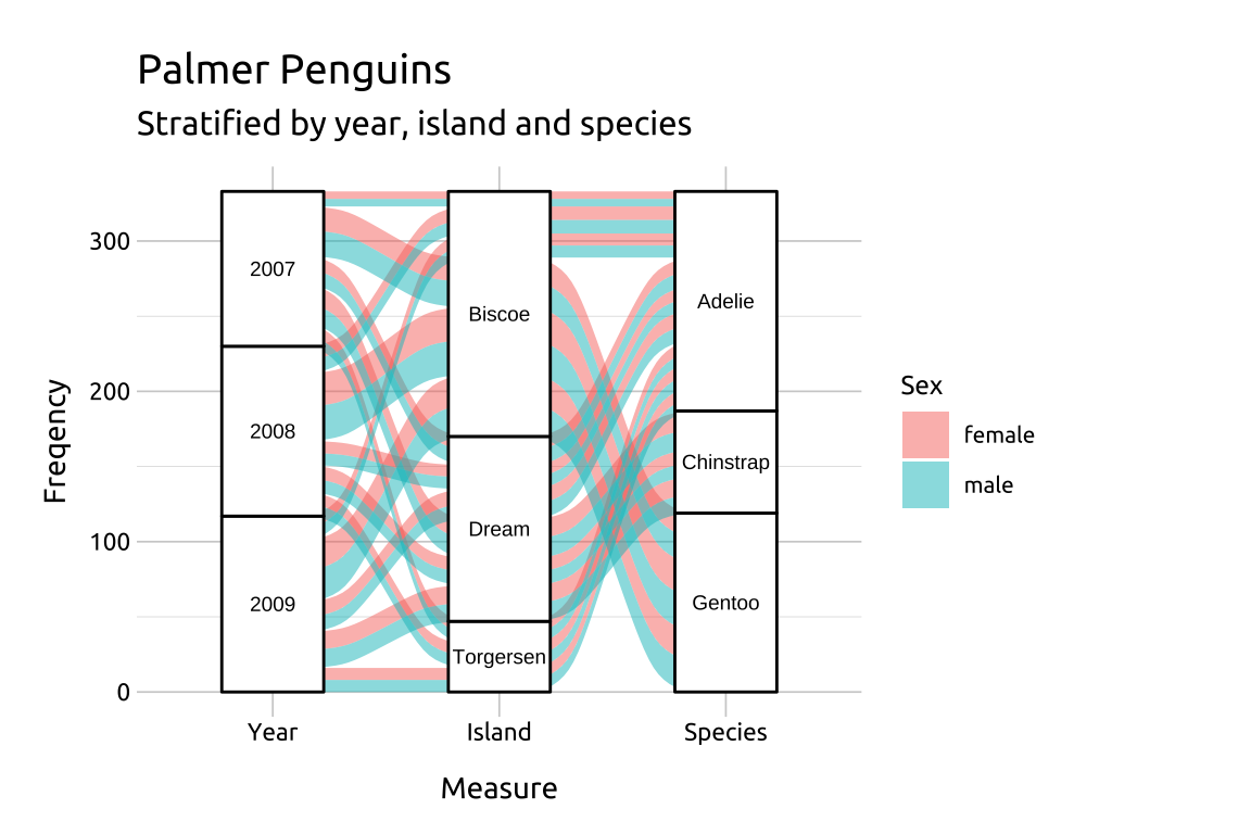

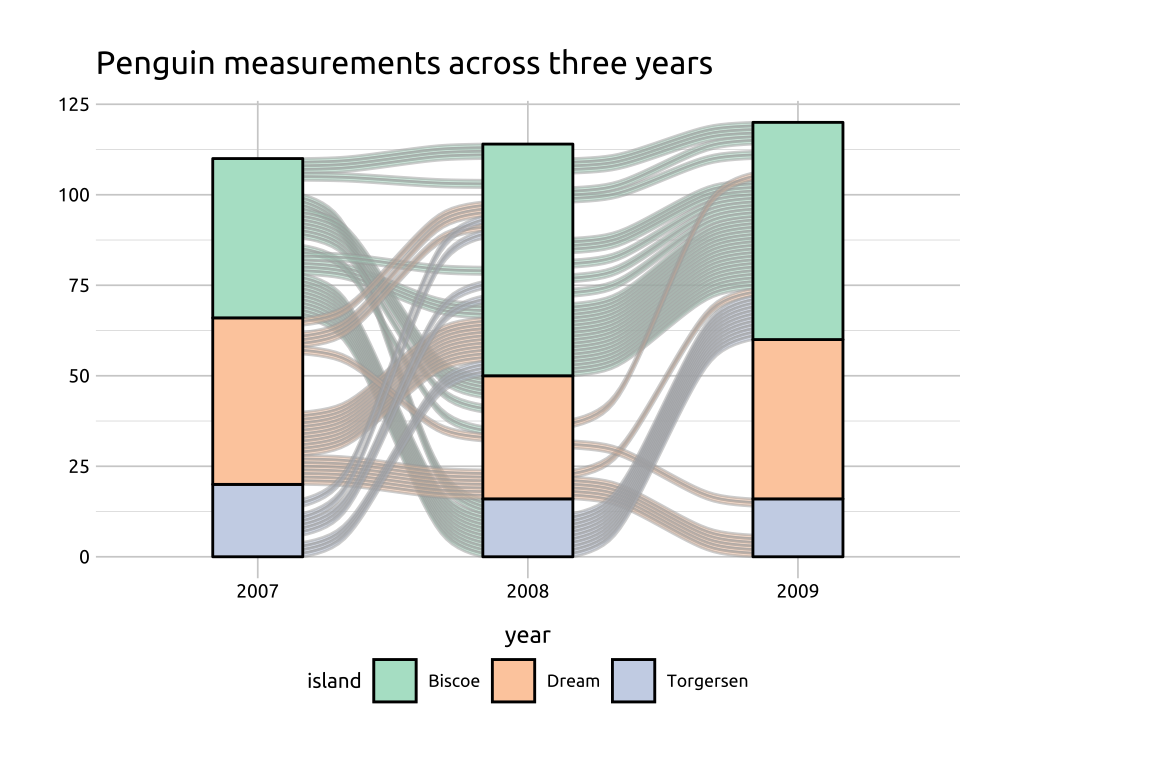
33.4.2 geom_flow()

If you’d like to arrange the date or time variable across the x, you can use the ggalluvial::geom_flow() with ggalluvial::geom_stratum().

• First create peng_alluvial, a subset of palmerpenguins::penguins_raw with all variables turned to factors.

peng_alluvial <- palmerpenguins::penguins_raw |> 
  janitor::clean_names() |> 
  dplyr::mutate(year = lubridate::year(date_egg),
         year = factor(year),
         individual_id = factor(individual_id),
         island = factor(island)) |> 
  dplyr::select(year, individual_id, island)
dplyr::glimpse(peng_alluvial)
#> Rows: 344
#> Columns: 3
#> $ year          <fct> 2007, 2007, 2007, 2007, 20…
#> $ individual_id <fct> N1A1, N1A2, N2A1, N2A2, N3…
#> $ island        <fct> Torgersen, Torgersen, Torg…

• Create labels with labs()

• Initiate graph with data

• Map the year to the x, island to stratum, individual_id to alluvium, island to fill, and island to label.

• Add scale_fill_brewer(), and set the type to "qual" and choose a palette

• Add the geom_flow(), with stat set to "alluvium", lode.guidance set to "frontback", and color to "#A9A9A9"

# labels
labs_alluvial <- labs(
  title = "Penguin measurements across three years")
# add geom_flow() 
ggp2_alluvial_flow <- ggplot(data = peng_alluvial,
  mapping = aes(x = year, stratum = island, 
    alluvium = individual_id, 
    fill = island, label = island)) +
  scale_fill_brewer(type = "qual", palette = "Pastel2") +
  geom_flow(stat = "alluvium",
    lode.guidance = "frontback",
    color = "#A9A9A9")

ggp2_alluvial_flow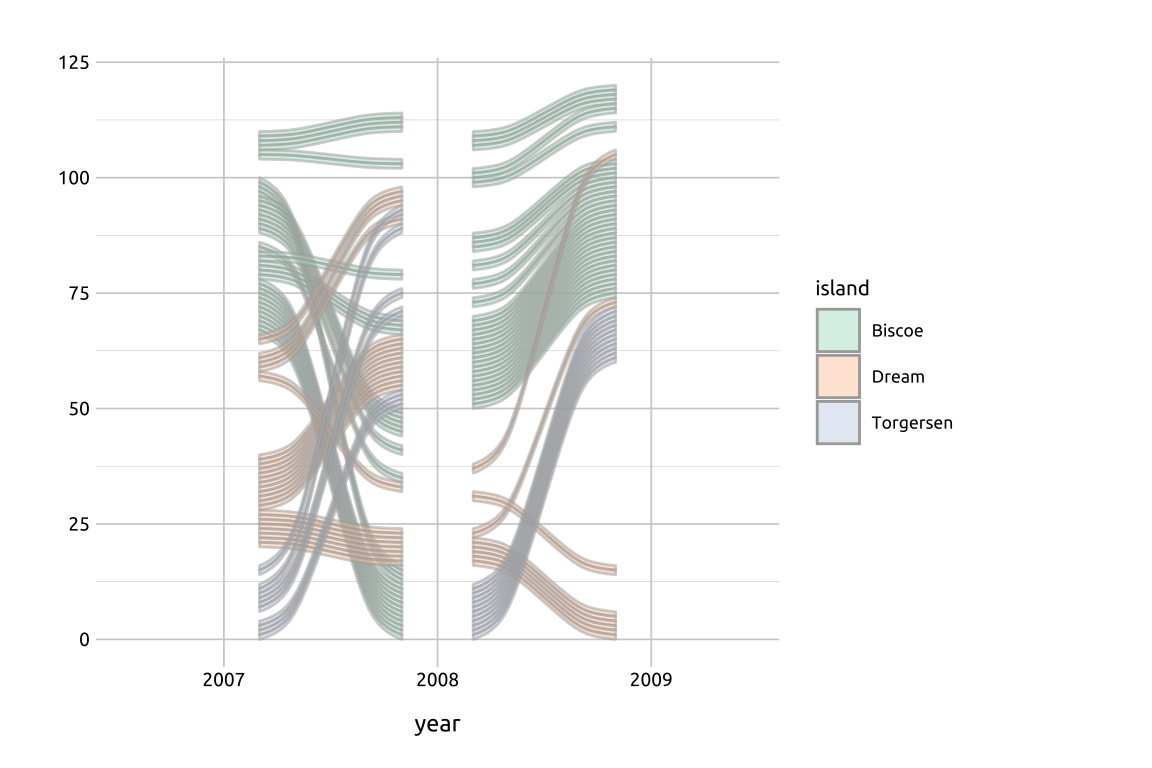

• Add ggalluvial::geom_stratum()

# add geom_stratum()
ggp2_alluvial_stratum <- ggp2_alluvial_flow +
  geom_stratum() 
ggp2_alluvial_stratum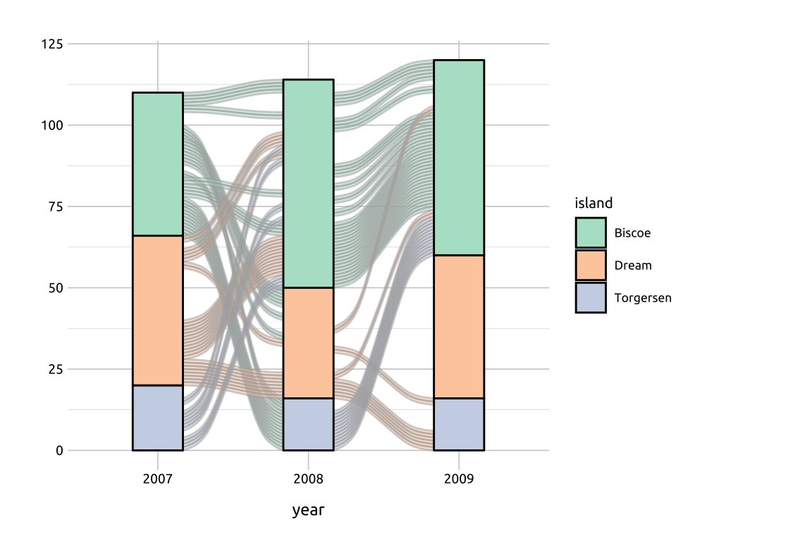

33.4.3 legend.position

Move legend to bottom with theme(legend.position = "bottom")

ggp2_alluvial_stratum + 
  labs_alluvial + 
  theme(legend.position = "bottom")