11 Heatmaps
11.1 Description
Heatmaps are color graphs that show data as a matrix with categories on the x and y axes. Each cell’s color corresponds to its value. They are useful for showing magnitude in two dimensions and often include a color scale. The intersecting cells contain variations of color saturation (i.e., the grade of purity or vividness) to represent the numerical values between groups.
Heatmap legends should be positioned on top or bottom and justified horizontally to preserve shape and improve readability.
11.2 Set up
PACKAGES:
Install packages.
show/hide
install.packages("fivethirtyeight")
library(fivethirtyeight)
library(ggplot2)
DATA:

For the heatmap, we’re going to re-structure and filter the bob_ross data from the fivethirtyeight package.
show/hide
heatmap_ross <- fivethirtyeight::bob_ross |>
pivot_longer(-c(episode, season,
episode_num, title),
names_to = "object",
values_to = "present") |>
mutate(present = as.logical(present),
object = str_replace_all(object, "_", " ")) |>
arrange(episode, object) |>
filter(object %in% c("conifer", "trees",
"tree", "snow", "palm trees", "grass",
"flowers", "cactus", "bushes", "cirrus",
"cumulus", "deciduous", "clouds", "fog")) |>
group_by(season, object) |>
summarise(occurrences = sum(present)) |>
ungroup()
#> `summarise()` has regrouped the output.
#> ℹ Summaries were computed grouped by season and
#> object.
#> ℹ Output is grouped by season.
#> ℹ Use `summarise(.groups = "drop_last")` to
#> silence this message.
#> ℹ Use `summarise(.by = c(season, object))` for
#> per-operation grouping (`?dplyr::dplyr_by`)
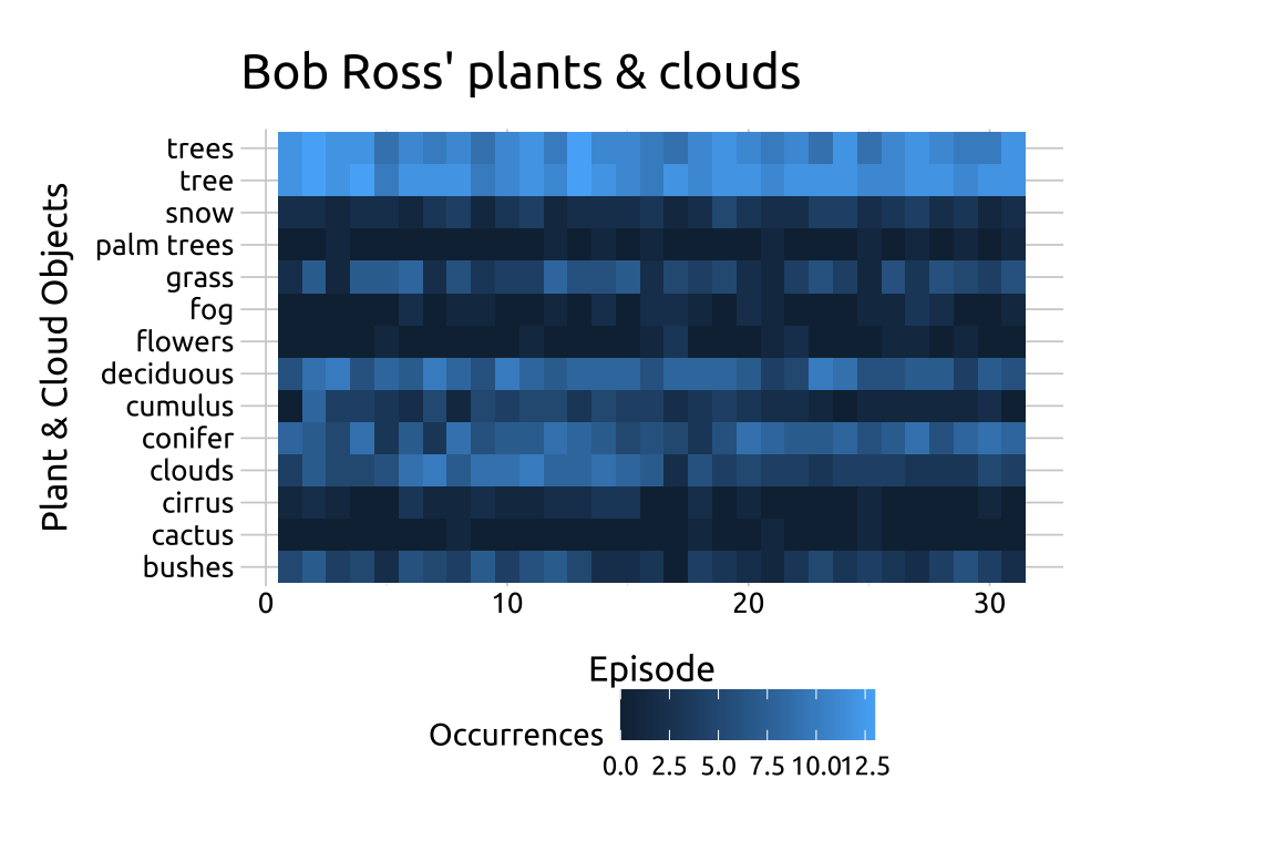
#> instead.11.3 Grammar
CODE:
Create labels with
labs()Initialize the graph with
ggplot()and providedataAssign
seasontox,objecttoy, andoccurrencestofillAdd the
geom_tile()Move the legend to the bottom with
theme(legend.position = "bottom")
show/hide
labs_heatmap_tile <- labs(
  title = "Bob Ross' plants & clouds",
  x = "Episode",
  y = "Plant & Cloud Objects",
  fill = "Occurrences")
ggp2_heatmap_tile <- ggplot(data = heatmap_ross,
       aes(x = season,
           y = object,
           fill = occurrences)) +
       geom_tile() +
    theme(legend.position = "bottom")
ggp2_heatmap_tile +
  labs_heatmap_tile
GRAPH:
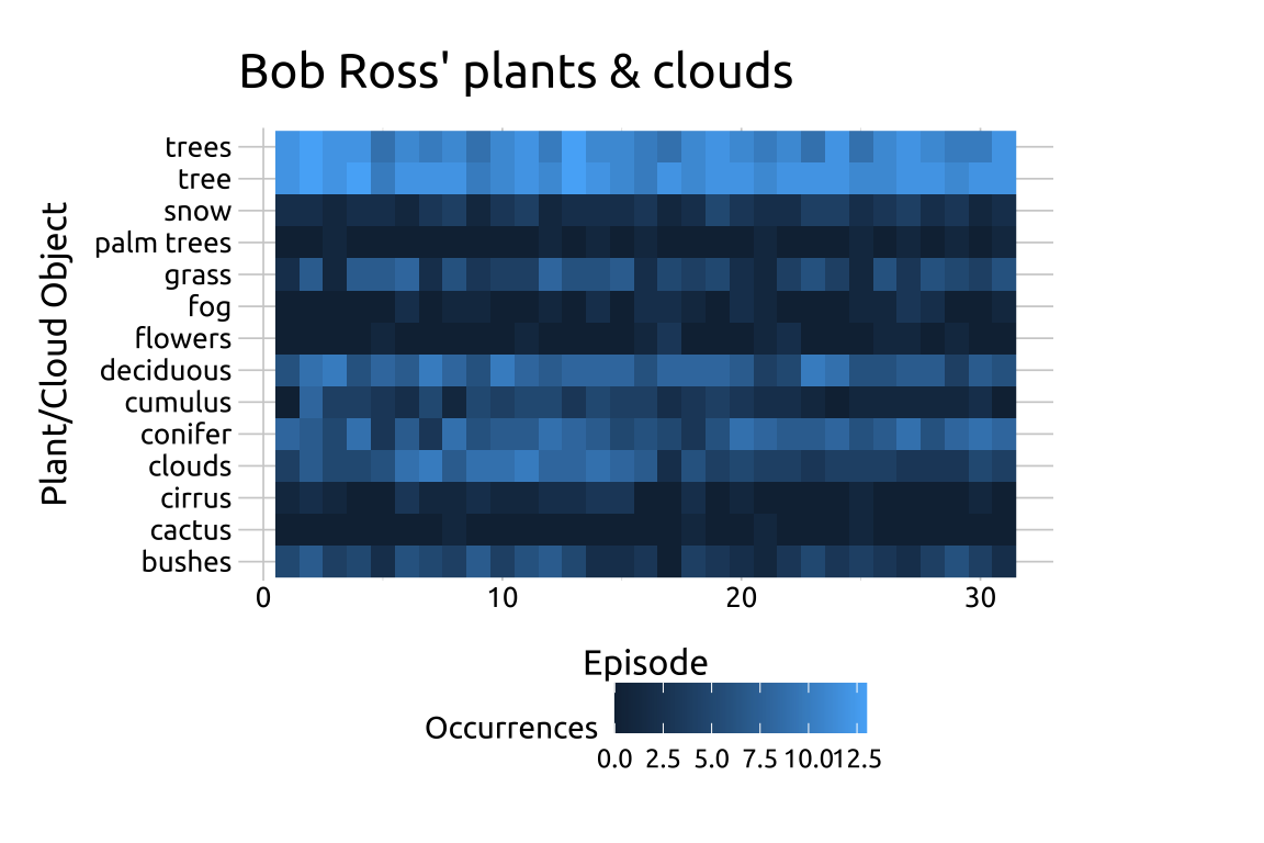
11.4 More info
In addition to geom_tile(), heatmaps can also be created with the geom_raster() function.
11.4.1 geom_raster()
Create labels with
labs()Initialize the graph with
ggplot()and providedataAssign
seasontox,objecttoy, andoccurrencesto fillAdd the
geom_raster()Move the legend to the bottom with
theme(legend.position = "bottom")
show/hide
labs_heatmap_raster <- labs(
  title = "Bob Ross' plants & clouds",
  x = "Episode",
  y = "Plant/Cloud Object",
  fill = "Occurrences")
ggp2_heatmap_raster <- ggplot(data = heatmap_ross,
       aes(x = season,
           y = object,
           fill = occurrences)) +
       geom_raster() +
    theme(legend.position = "bottom")
ggp2_heatmap_raster +
  labs_heatmap_raster