42  Hexagon bins

This graph is largely complete and just needs final proof reading.

This graph requires:

✅ two numeric (continuous) variable

42.1 Description

Hexagon bins (or hex-bins) are a very similar to 2-D histograms, but instead of dividing the graph area into a grid, it’s divided into hexagons. The number of points inside each per hexagon determine it’s color.

42.2 Set up

PACKAGES:

Install packages.

install.packages("palmerpenguins")
library(palmerpenguins)
library(ggplot2)

DATA:

Artwork by allison horst

We’ll take the flipper_length_mm, bill_length_mm, bill_depth_mm, species, sex, and island variables from palmerpenguins::penguins and drop the missing values.

penguins_hex <- palmerpenguins::penguins |> 
    dplyr::select(flipper_length_mm, bill_depth_mm,
        bill_length_mm, species, sex, island) |> 
    tidyr::drop_na()
glimpse(penguins_hex)
#> Rows: 333
#> Columns: 6
#> $ flipper_length_mm <int> 181, 186, 195, 193, 19…
#> $ bill_depth_mm     <dbl> 18.7, 17.4, 18.0, 19.3…
#> $ bill_length_mm    <dbl> 39.1, 39.5, 40.3, 36.7…
#> $ species           <fct> Adelie, Adelie, Adelie…
#> $ sex               <fct> male, female, female, …
#> $ island            <fct> Torgersen, Torgersen, …

42.3 Grammar

CODE:

• Create labels with labs()

• Initialize the graph with ggplot() and provide data

• Map bill_length_mm to the x and flipper_length_mm to the y

• Add the geom_hex() layer

labs_hex <- labs(
    title = "Adult Foraging Penguins", 
    subtitle = "Near Palmer Station, Antarctica", 
    x = "Bill length (mm)", 
    y = "Flipper length (mm)")
# graph
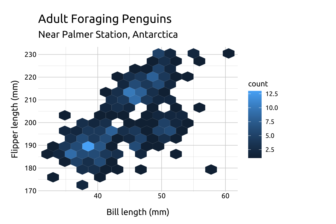
ggp2_hex <- ggplot(data = penguins_hex, 
    aes(x = bill_length_mm, y = flipper_length_mm)) + 
    geom_hex()

ggp2_hex + 
    labs_hex

GRAPH:

42.4 More info

42.4.1 Bins

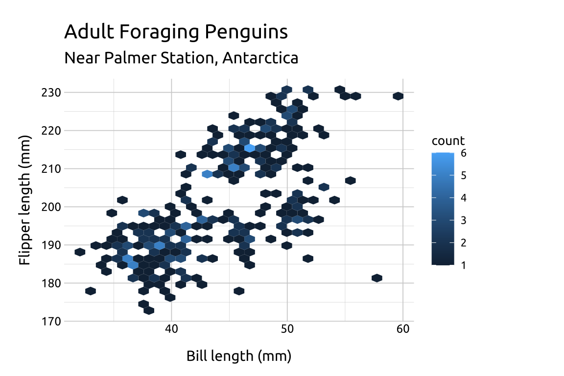
Below we change the bins to 20 and 15 and save these layers as ggp2_hex_b20 and ggp2_hex_b15.

Decreasing the number of bins increases the size of the hexagons (and makes them larger).

ggp2_hex_b20 <- ggplot(data = penguins_hex,
    aes(x = bill_length_mm, y = flipper_length_mm)) +
    geom_hex(bins = 20)
ggp2_hex_b20 +
    labs_hex


ggp2_hex_b15 <- ggplot(data = penguins_hex,
    aes(x = bill_length_mm, y = flipper_length_mm)) +
    geom_hex(bins = 15)
ggp2_hex_b15 +
    labs_hex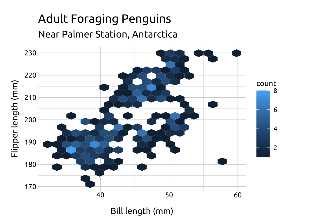

42.4.2 Scale

• We can adjust the color scale using scale_color_discrete_sequential() and setting aesthetics to "fill".

• If the hexagons overlap, we can use the alpha to make them slightly transparent.

labs_hex2 <- labs(
    title = "Adult Foraging Penguins", 
    subtitle = "Near Palmer Station, Antarctica", 
    x = "Bill length (mm)", 
    y = "Flipper length (mm)",
    fill = "Sex")
ggplot(data = penguins_hex, 
    aes(x = bill_length_mm, 
        y = flipper_length_mm)) + 
    geom_hex(aes(fill = sex), 
             bins = 15, 
             alpha = 3/4) + 
    scale_color_discrete_sequential(
        aesthetics = "fill", 
        rev = FALSE,
        palette = "Viridis") +
    labs_hex2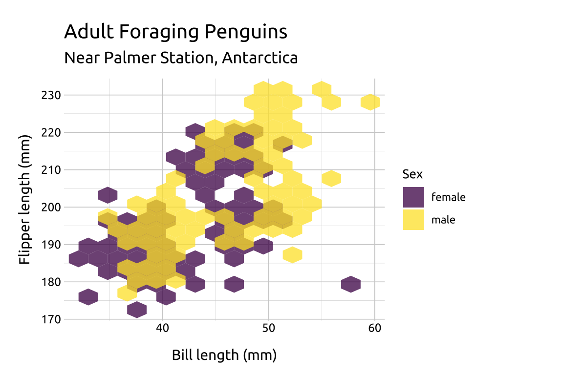

Get a full list of available color palette’s using hcl_palettes(type = "sequential")

42.4.3 Options

• binwidth allows us to manually adjust the size of the hexagons.

• linewidth is also helpful when using alpha for overlapping values.

labs_hex3 <- labs(
    title = "Adult Foraging Penguins", 
    subtitle = "Near Palmer Station, Antarctica", 
    x = "Bill length (mm)", 
    y = "Flipper length (mm)",
    fill = "Species")

ggplot(data = penguins_hex, 
    aes(x = bill_length_mm, 
        y = flipper_length_mm, 
        fill = species)) + 
    geom_hex(binwidth = c(1.1, 3),
        linewidth = 0.5, 
        alpha = 3/4,
        color = "#000000") + 
    scale_color_discrete_sequential(
        aesthetics = "fill", 
        palette = "Dark Mint") +
    labs_hex3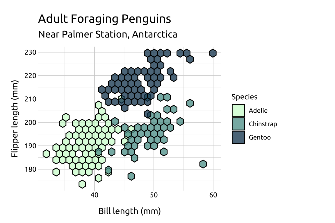

Bins can be set with bins (a single number) or binwidth (a numeric vector of c(x, y))