41  2D histograms

This graph is largely complete and just needs final proof reading.

This graph requires:

✅ two numeric (continuous) variables

41.1 Description

Standard histograms separate a variable’s values into discrete groups, or ‘bins,’ which are arranged in increasing order across the x axis. The y axis displays the frequency (or count) of values within each bin.

Vertical bars capture the variable’s distribution using the height of the bar to represent the number of values per ‘bin’, and the number of bars corresponds with the bin value (or ‘bin-width’).

When we extend this display to two numerical/quantitative variables, the bins are used to divide the total graph area into a grid, and color is used to display the variation in frequency (or count) of both variable values that fall within each intersecting square.

41.2 Set up

PACKAGES:

Install packages.

install.packages("palmerpenguins")
library(palmerpenguins)
library(ggplot2)

DATA:

Artwork by allison horst

We’ll take the flipper_length_mm, bill_length_mm, and species variables from palmerpenguins::penguins and drop the missing values.

penguins_2dhist <- palmerpenguins::penguins |> 
    dplyr::select(flipper_length_mm, bill_length_mm, 
                  sex, species, body_mass_g) |> 
    tidyr::drop_na()
glimpse(penguins_2dhist)
#> Rows: 333
#> Columns: 5
#> $ flipper_length_mm <int> 181, 186, 195, 193, 19…
#> $ bill_length_mm    <dbl> 39.1, 39.5, 40.3, 36.7…
#> $ sex               <fct> male, female, female, …
#> $ species           <fct> Adelie, Adelie, Adelie…
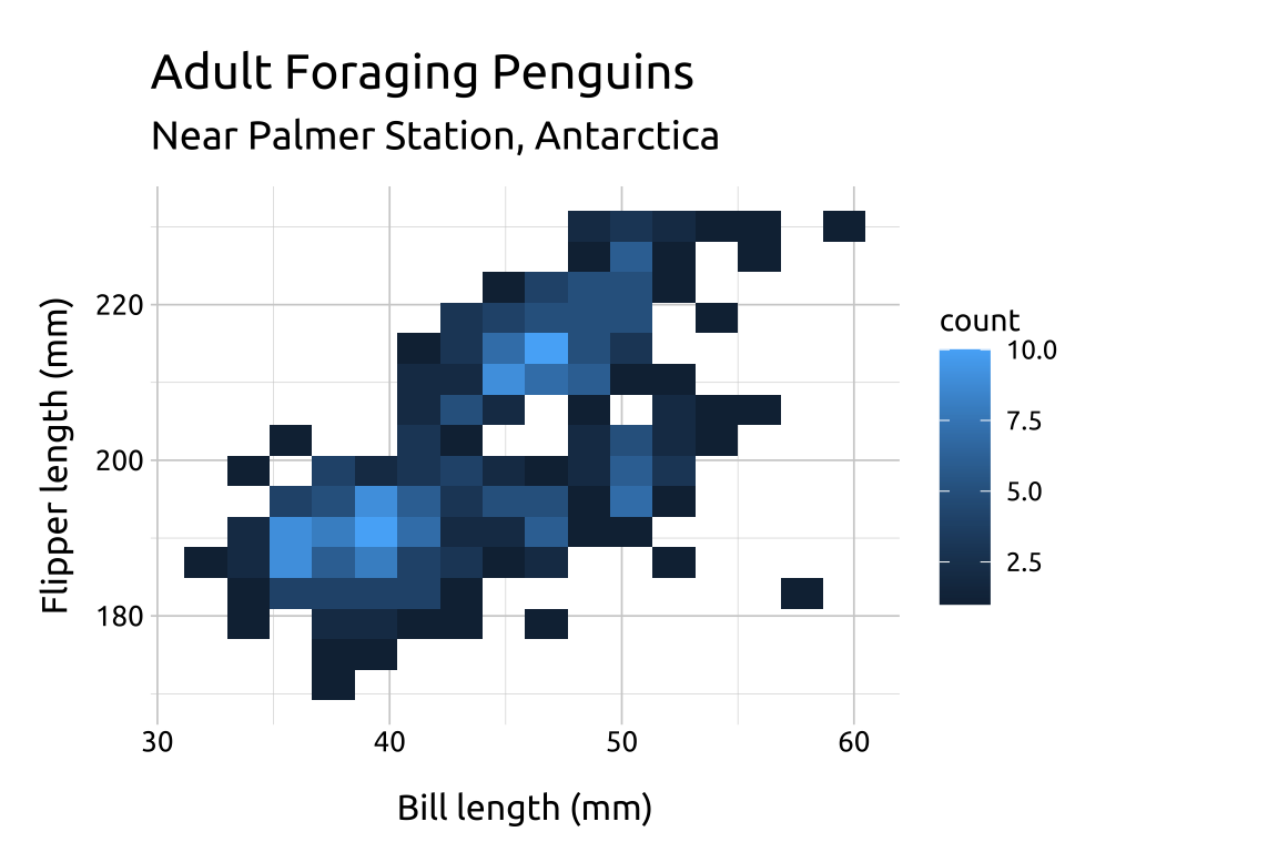
#> $ body_mass_g       <int> 3750, 3800, 3250, 3450…

41.3 Grammar

CODE:

• Create labels with labs()

• Initialize the graph with ggplot() and provide data

• Map bill_length_mm to the x and flipper_length_mm to the y

• Add the geom_bin2d() layer

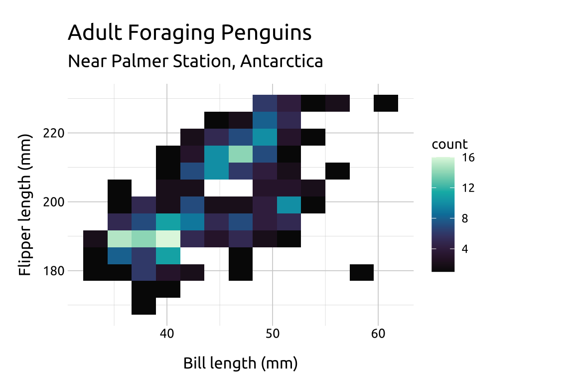
labs_2dhist <- labs(
    title = "Adult Foraging Penguins", 
    subtitle = "Near Palmer Station, Antarctica", 
    x = "Bill length (mm)", 
    y = "Flipper length (mm)")

ggp2_2dhist <- ggplot(data = penguins_2dhist, 
    mapping = aes(x = bill_length_mm, 
                  y = flipper_length_mm)) + 
    geom_bin2d(bins = 15)
            
ggp2_2dhist + 
    labs_2dhist

GRAPH:

41.4 More info

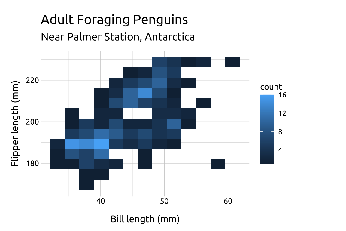
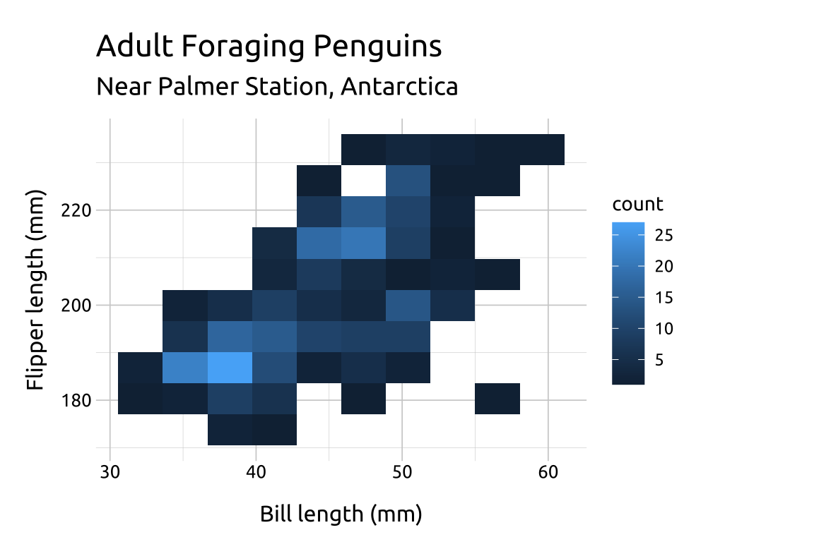
41.4.1 Bins

The value for bins will be vary depending on the variable values–there is no correct number:

• If the number of bins is too low, the density may hide important nuances between the variables.

• If the number of bins is too high, the noise might drown out the signal.

• Below we change the bins to 9, 12 and 18 to compare the display:

ggp2_base <- ggplot(data = penguins_2dhist, 
    mapping = aes(x = bill_length_mm, 
                  y = flipper_length_mm))

ggp2_2dhist_bins18 <- ggp2_base + 
                    geom_bin2d(bins = 18)

ggp2_2dhist_bins12 <- ggp2_base + 
                    geom_bin2d(bins = 12) 

ggp2_2dhist_bins9 <- ggp2_base + 
                    geom_bin2d(bins = 9)

ggp2_2dhist_bins18 + 
     labs_2dhist 

ggp2_2dhist + 
    labs_2dhist

ggp2_2dhist_bins12 + 
     labs_2dhist 

ggp2_2dhist_bins9 + 
  labs_2dhist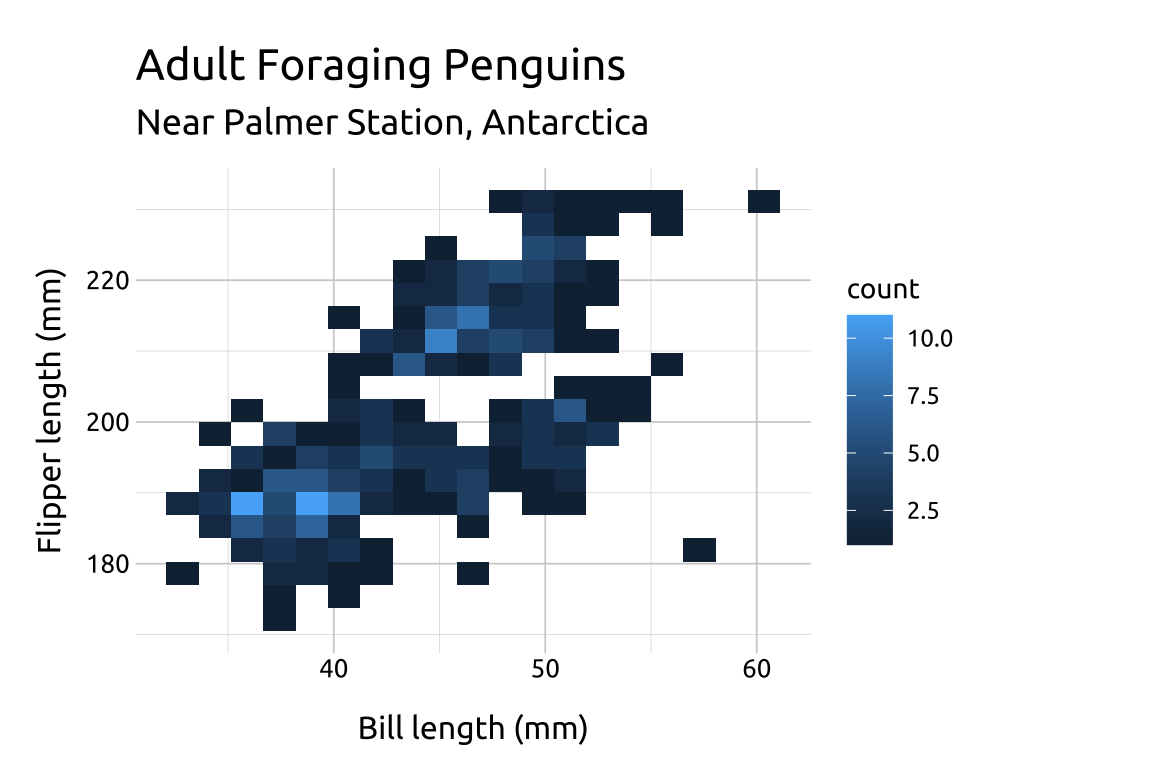

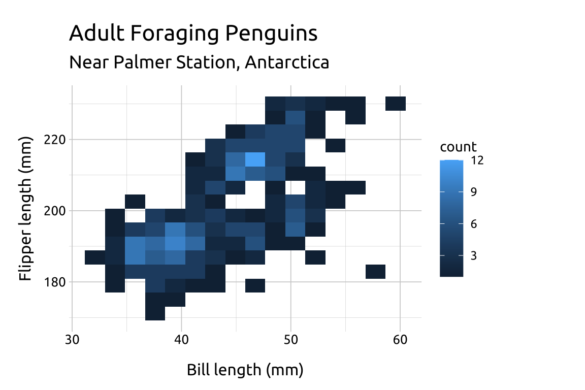
41.4.2 Scale

scale_fill_continuous_sequential() comes with a variety of palettes to choose from (run hcl_palettes(type = "sequential") to view the full list).

We can also reverse the order of the fill color scale with rev (TRUE or FALSE).

ggp2_2dhist_bins12 + 
    scale_fill_continuous_sequential(
        palette = "Mako", 
        rev = TRUE) +
    labs_2dhist 

ggp2_2dhist_bins12 + 
    scale_fill_continuous_sequential(
        palette = "Mako", 
        rev = FALSE) +
    labs_2dhist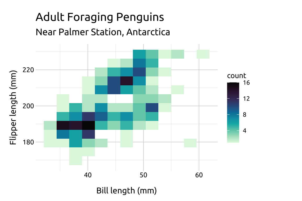 

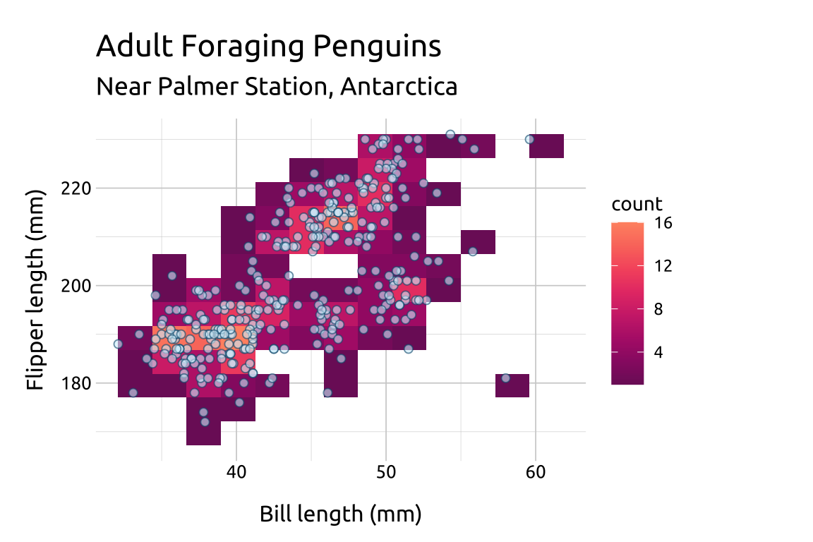
41.4.3 Options

If you set the point shape to 21, you have control over both color and fill.

In the previous example we showed how to reverse the color scale for the palette in scale_fill_continuous_sequential().

• Below we reverse the color scale, but also manually set which colors on the scale we want to begin with (i.e., smallest data value) and which color we want to end with (i.e., the largest data value). Possible values range from 0 - 1.

• We also add a geom_point() layer.

ggp2_2dhist_bins12 +
  scale_fill_continuous_sequential(
    palette = "SunsetDark",
    rev = TRUE,
    begin = 1.0,
    end = 0.3) +
  geom_point(
    fill = "#D4F0FC",
    color = "#02577A",
    shape = 21,
    size = 1.8,
    alpha = 0.60) +
  labs_2dhist