39 Parallel sets
39.1 Description
Parallel sets (also referred to as Sankey diagrams or Alluvial charts) show the counts of categorical variables connected via a two-sided parallel display (or ‘sets’). Parallel sets can also be used to show different states of paired dependent relationships (such as input vs output), or time 1 vs time 2.
The height of the connecting bands between the categories on the x axis represent the relative counts for each discrete level (displayed on the y axis). The levels within each variable are represented with color.
We can build parallel set diagrams with the ggforce package.
Also check out alluvial charts.
39.2 Set up
PACKAGES:
Install packages.
show/hide
# pak::pak("thomasp85/ggforce")
install.packages("palmerpenguins")
library(ggforce)
library(palmerpenguins)
library(ggplot2)
DATA:
We’re going to remove the missing values from palmerpenguins::penguins, count the categorical variables (island, sex, species), and rename the n column (produced by the count() function) to value.
ggforcehas a specialgather_set_data()function that changes tidy data into a tidy(er) format
show/hide
peng_wide <- palmerpenguins::penguins |>
  drop_na() |>
  count(island, species, sex) |>
  rename(value = n)
para_set_peng <- ggforce::gather_set_data(
                            data = peng_wide,
                            x = 1:3)
dplyr::glimpse(para_set_peng)
#> Rows: 30
#> Columns: 7
#> $ island  <fct> Biscoe, Biscoe, Biscoe, Biscoe, …
#> $ species <fct> Adelie, Adelie, Gentoo, Gentoo, …
#> $ sex     <fct> female, male, female, male, fema…
#> $ value   <int> 22, 22, 58, 61, 27, 28, 34, 34, …
#> $ id      <int> 1, 2, 3, 4, 5, 6, 7, 8, 9, 10, 1…
#> $ x       <chr> "island", "island", "island", "i…
#> $ y       <fct> Biscoe, Biscoe, Biscoe, Biscoe, …
39.3 Grammar
CODE:
Create labels with
labs()Initialize the graph with
ggplot()and providedataMap
xtox,idtoid,ytosplit, andvaluetovalueIn the
geom_parallel_sets()function, mapsextofilland manually set thealpha(opacity) and theaxis.widthIn the
geom_parallel_sets_axes()function, set theaxis.widthto the same value as thegeom_parallel_sets()aboveFor labeling, adjust the
sizemanually and set thecolorto something that stands out against the black vertical axesManually label the
xaxis withscale_x_continuous(), setting thebreaksandlabelsto the variable names in thepeng_widedatasetFinally, remove the
xtitle withaxis.title.x = element_blank()
show/hide
labs_psets <- labs(
title = "Categories of Palmer Penguins",
y = "Count", fill = "Sex")
ggp2_psets <- ggplot(data = para_set_peng,
mapping = aes(x = x,
id = id,
split = y,
value = value)) +
geom_parallel_sets(aes(fill = sex),
alpha = 0.3,
axis.width = 0.07)
ggp2_psets_axes <- ggp2_psets +
geom_parallel_sets_axes(
axis.width = 0.07)
ggp2_psets_labs <- ggp2_psets_axes +
geom_parallel_sets_labels(
size = 2.0,
color = '#ffffff') +
scale_x_discrete(
labels = c(island = "Island", species = "Species", sex = "Sex")) +
theme(axis.title.x = element_blank())
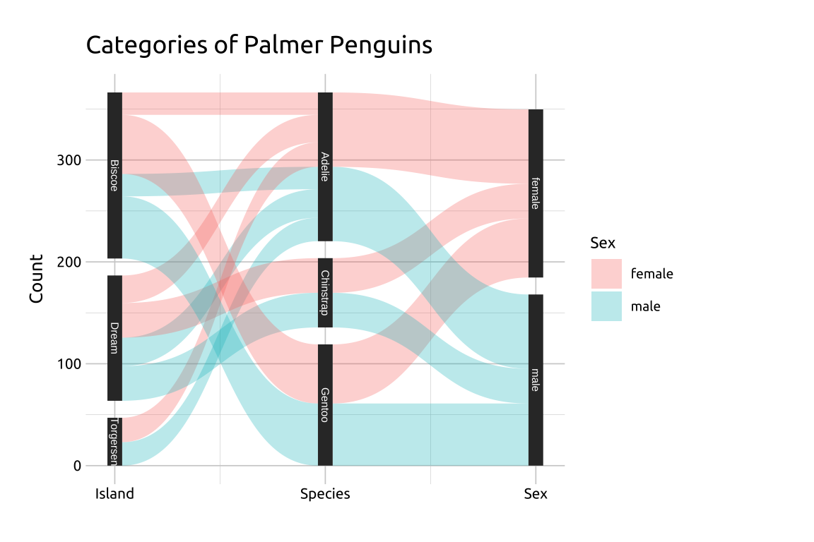
ggp2_psets_labs +
labs_psetsGRAPH:

39.4 More info
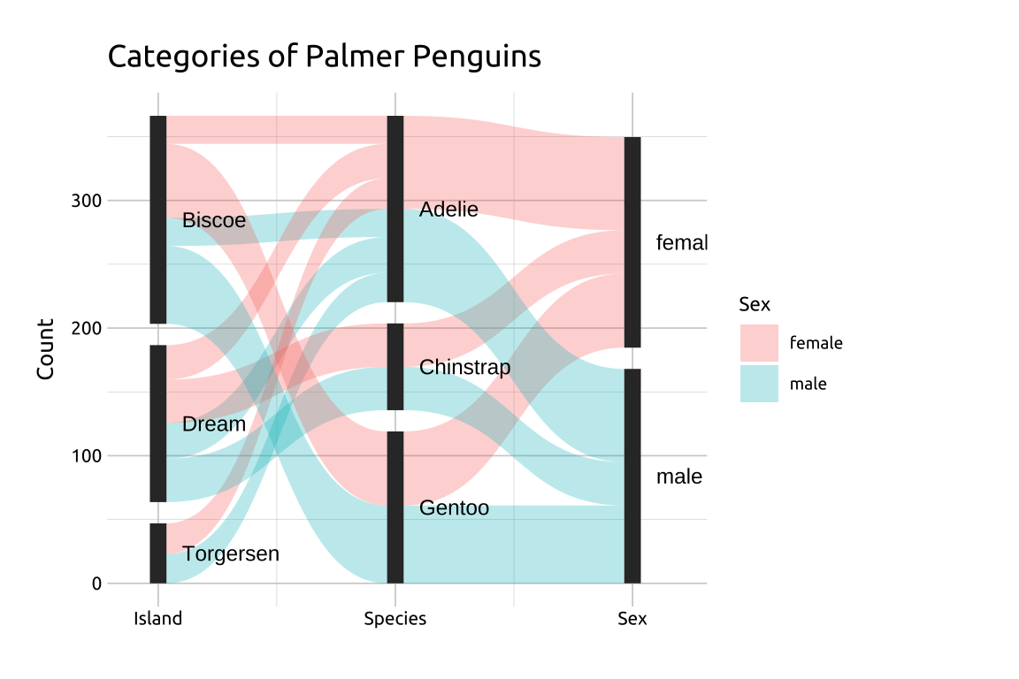
If the categories have long names, you can move the location of the labels outside the set.
39.4.1 Labeling sets
If the categories have long names, use the angle, nudge_x/nudge_y and hjust/vjust in geom_parallel_sets_labels() to adjust the size, location, and color of the labels.
- Manually setting the
limitsof thexaxis inscale_x_continuous()will also give more room for the labels.
show/hide
ggp2_psets_axes +
  geom_parallel_sets_labels(
      size = 3.2,
      colour = '#000000',
      angle = 0,
      nudge_x = 0.1,
      hjust = 0) +
  scale_x_discrete(
        labels = c(island = "Island", species = "Species", sex = "Sex"),
        expand = expansion(add = c(0.1, 0.4))) +
  theme(axis.title.x = element_blank()) +
    labs_psets