19 Overlapping histograms
19.1 Description
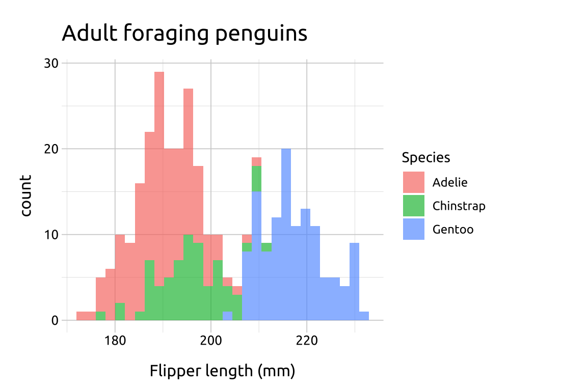
Overlapping histograms allow us to compare distributions across the groups of a categorical (or ordinal) variable.
19.2 Set up
PACKAGES:
Install packages.
show/hide
install.packages("palmerpenguins")
library(palmerpenguins)
library(ggplot2)
DATA:
The penguins data.
show/hide
penguins <- palmerpenguins::penguins
glimpse(penguins)
#> Rows: 344
#> Columns: 8
#> $ species           <fct> Adelie, Adelie, Adelie…
#> $ island            <fct> Torgersen, Torgersen, …
#> $ bill_length_mm    <dbl> 39.1, 39.5, 40.3, NA, …
#> $ bill_depth_mm     <dbl> 18.7, 17.4, 18.0, NA, …
#> $ flipper_length_mm <int> 181, 186, 195, NA, 193…
#> $ body_mass_g       <int> 3750, 3800, 3250, NA, …
#> $ sex               <fct> male, female, female, …
#> $ year              <int> 2007, 2007, 2007, 2007…
19.3 Grammar
CODE:
Create labels with
labs()Initialize the graph with
ggplot()and providedataMap
flipper_length_mmto thexaxis andspeciestofillSet
alphato2/3insidegeom_histogram()
show/hide
labs_ovrlp_hist <- labs(
  title = "Adult foraging penguins",
  x = "Flipper length (mm)",
  fill = "Species")
ggp2_ovrlp_hist <- ggplot(data = penguins,
     aes(x = flipper_length_mm,
         fill = species)) +
     geom_histogram(alpha = 2/3)
ggp2_ovrlp_hist +
  labs_ovrlp_hist
Experiment with different binwidths when comparing distributions across groups.
GRAPH:
Histograms work by dividing the variable provided to x into bins and counting the number of observations in each bin.
