Introduction

Caution

This section is still being developed. The contents are subject to change.

ggplot2 syntax

“making infinite use of finite means” - Wilhelm von Humboldt

Grammar is often defined as the system of rules for any given language and includes word meanings, internal structures, and word arrangement. Syntax is the form, structure and order for constructing statements. ggplot2‘s syntax is built on the grammar & syntax of R. In R, objects are like nouns, and functions are like verbs (i.e., functions ’do things’ to objects).

The ggplot2 syntax is comprised of layers, which we can use as templates to build increasing customize and complex graphs.

The Data Layer

The data layer consists of a rectangular object (like a spreadsheet) with columns and rows:

# drop missing values
penguins <- tidyr::drop_na(penguins)
ggplot(data = penguins)

The Mapping Layer

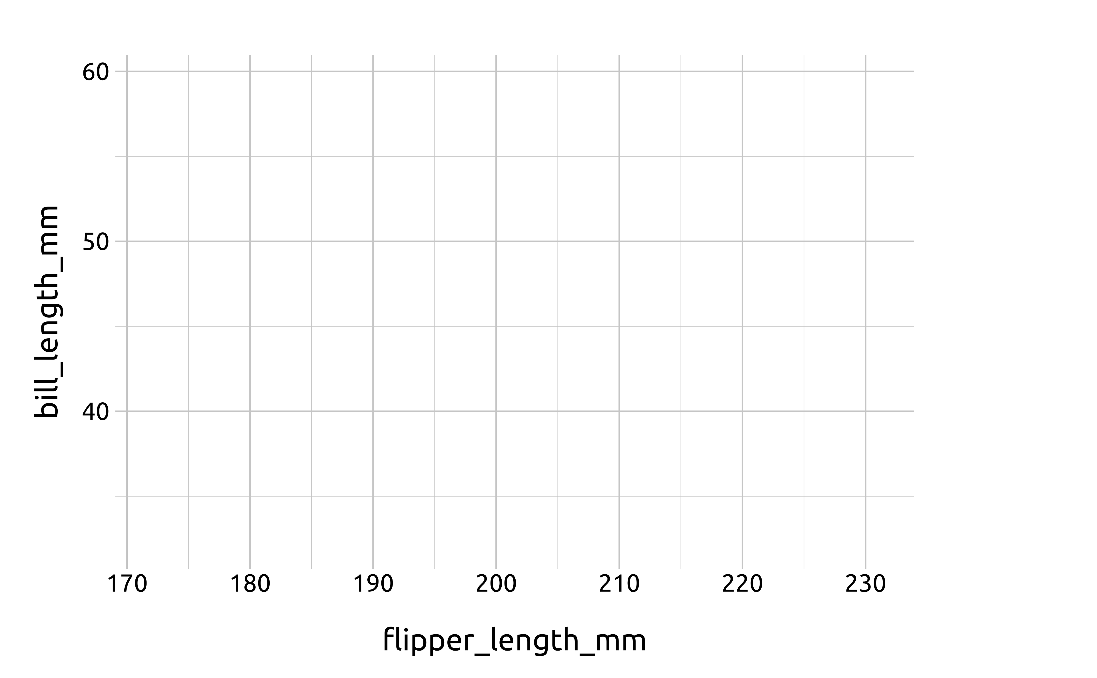
The mapping layer assigns columns (variables) from the data to a visual property (i.e. graph ’aes’ thetic)

ggplot(data = penguins,
  mapping = 
    aes(
      x = flipper_length_mm, y = bill_length_mm
      )
  )

Basic Template: Data, aesthetic mappings, geom

ggplot(data = <DATA>) +
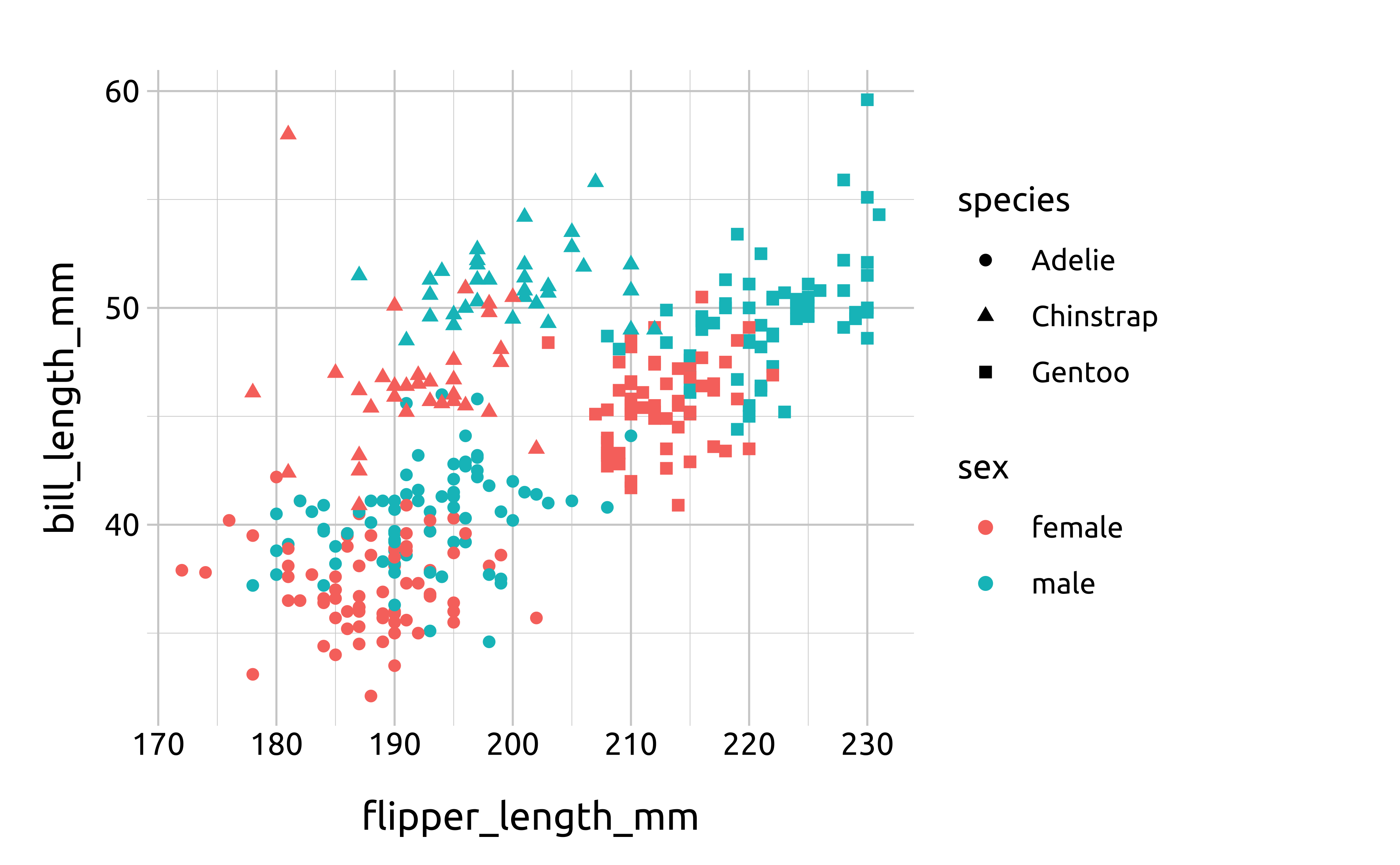
  geom_*(mapping = aes(<AESTHETIC MAPPINGS>))

The Stats/Geoms Layer

geom_*() functions include statistical transformations, shapes, and position adjustments for how to ‘draw’ the data on the graph

ggplot(data = penguins,
  mapping = aes(
    x = flipper_length_mm, y = bill_length_mm
    )
  ) +
  geom_point(
    aes(
      shape = species, color = sex
      )
    )

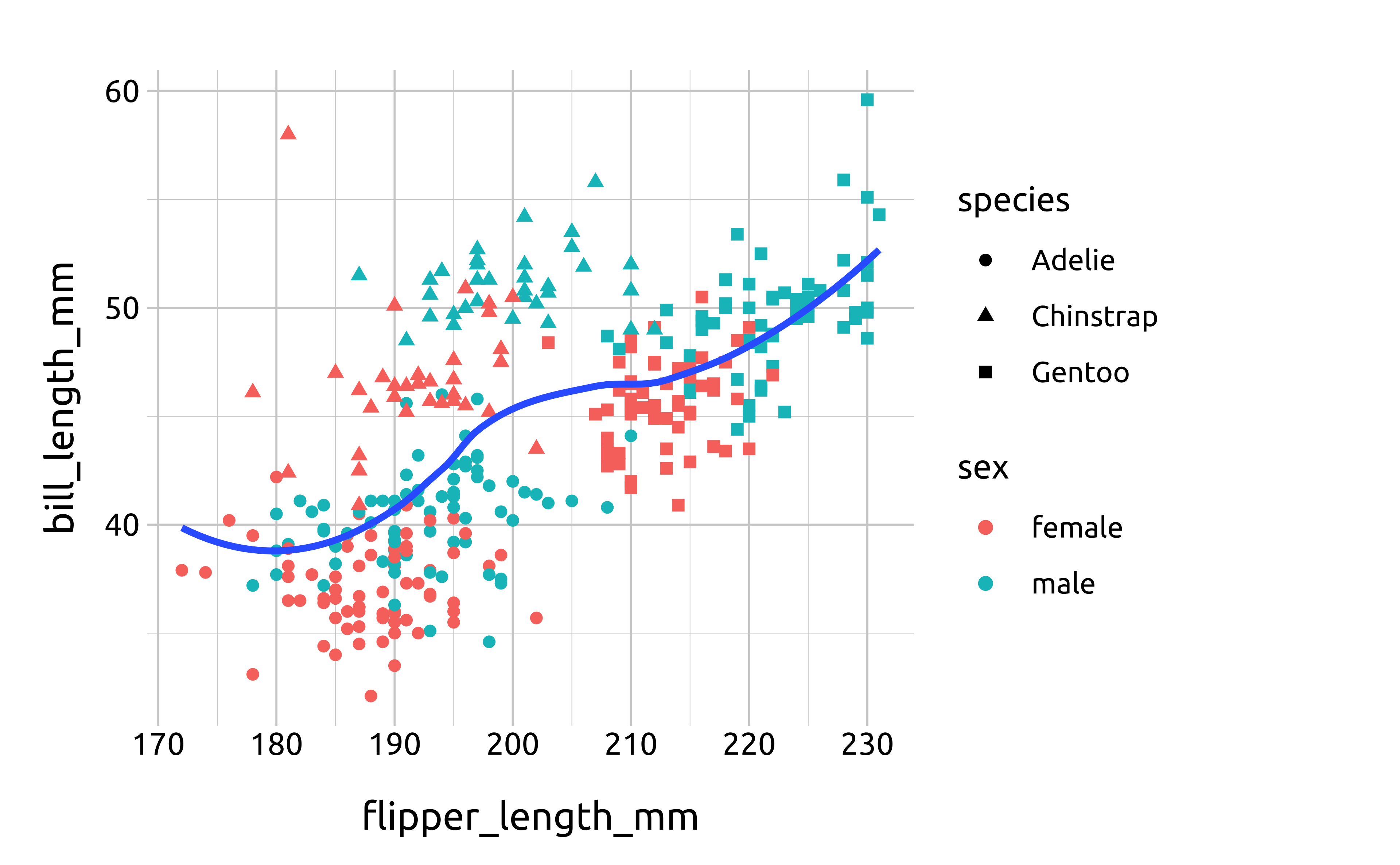
We can have multiple layers (data, mappings, geoms) in a single graph.

ggplot(data = penguins,
 # layer 1
  mapping = aes(
    x = flipper_length_mm, y = bill_length_mm
    )
  ) +
  geom_point(
    aes(
      shape = species, color = sex
      )
    ) +
# layer 2
  geom_smooth(
    mapping = aes(
      x = flipper_length_mm, y = bill_length_mm), 
        se = FALSE
    )

• Template + 1 Layer: more geoms and more aesthetic mappings

ggplot(data = <DATA>) +
    geom_*(mapping = aes(<AESTHETIC MAPPINGS>)) +
    geom_*(mapping = aes(<AESTHETIC MAPPINGS>))

Position, Labels & Themes

With a finite number of objects & functions, we can combine ggplot2’s grammar and syntax to create an infinite number of graphs!

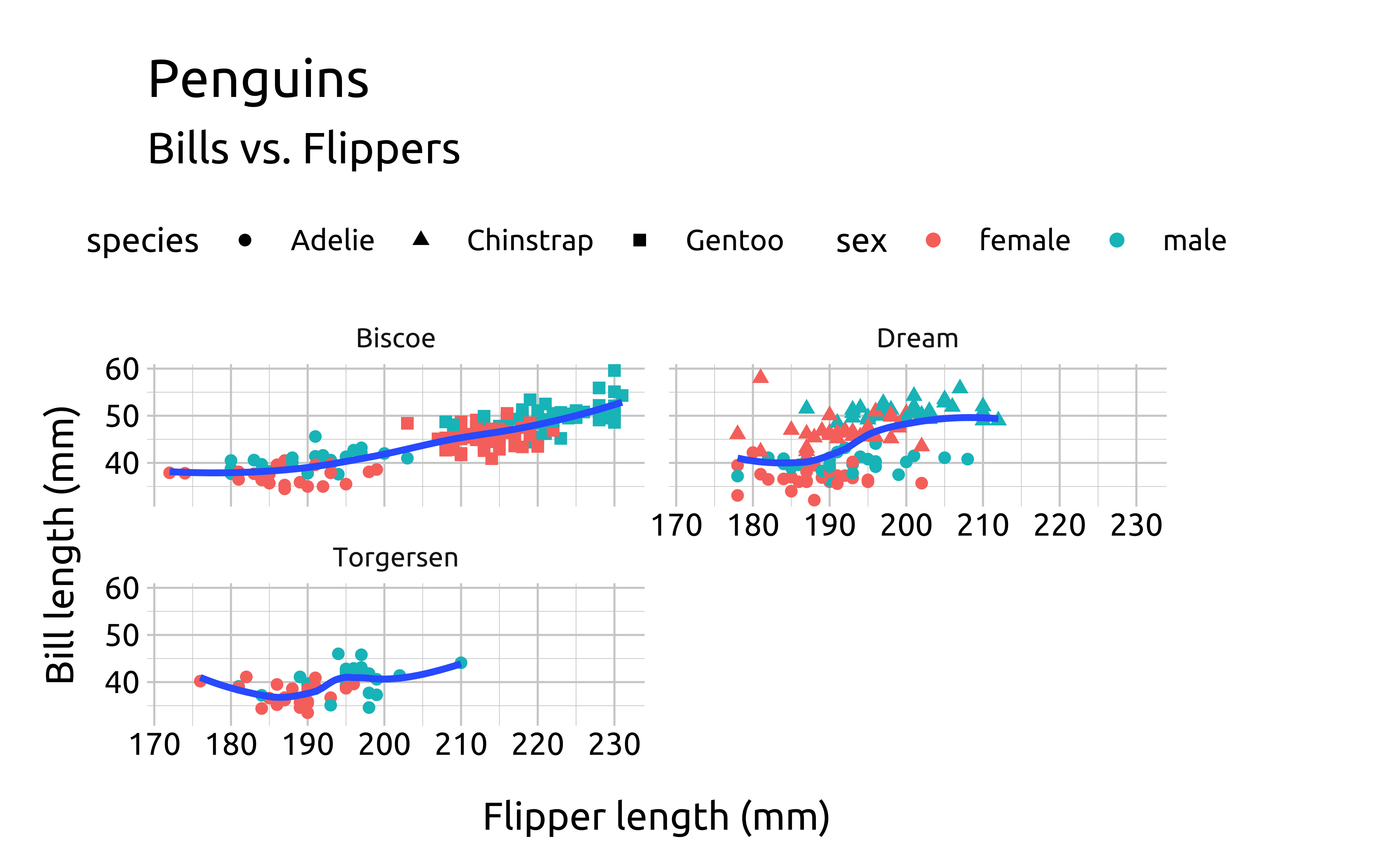
ggplot(data = penguins,
 # layer 1
  mapping = aes(
    x = flipper_length_mm, y = bill_length_mm
    )
  ) +
  geom_point(
    aes(
      shape = species, color = sex
      )
    ) +
# layer 2
  geom_smooth(
    mapping = aes(
      x = flipper_length_mm, y = bill_length_mm), 
        se = FALSE
    ) +
# layer 3
  facet_wrap(
    . ~ island, ncol = 2
    ) + 
  # labels
  labs(
    x = 'Flipper length (mm)', y = 'Bill length (mm)', 
    title = 'Penguins',  subtitle = 'Bills vs. Flippers'
    ) + 
  # themes
  theme(legend.position = "top") 

Template + 2 Layers + Facets + Theme + Labels

Layers = infinitely extensible!

ggplot(data = <DATA>) +
    geom_*(mapping = aes(<AESTHETIC MAPPINGS>)) +
    geom_*(mapping = aes(<AESTHETIC MAPPINGS>)) +
    facet_* +
    theme() +
    labs()

Graph Categories

Graphs have been categorized into the following types (you can see them in the floating table of contents to your left).

• Univariate: if you have a single column you’re trying to visualize

• Amounts: counts or simple summary statistics of one or two columns in a dataset

• Proportions: ratio displays of part-to-whole

• Distributions: displaying the shape of a variable’s values (normalcy, skewness, kurtosis, etc.)

• Dates & Times: changes in quantitative or categorical variables over a dimension of time (date-time, date, year, month, quarter, etc.).

• Relationships: how does the change of values in variable x affect the values in variable y (and possibly z)?

Some graphs can justifiably belong to more than one category, and wherever this is the case, I’ve tried to include links to other applications in the notes.

Assumptions

I’ve made an effort to write the graph code so it can be read and understood without having to execute it.¹ However, the examples assume the reader has already answered the question, “what kind of data do I have?”²

Style & structure

Each graph has the following sections:

1. Prerequisites

   • Should I use this graph?
     
   • This graph requires:
     

2. Description

   • A brief summary of the graph’s background, purpose, and aesthetics.

3. Set up

   • Packages
     • Code for installing development version of packages (if necessary) for graphs and data.
   • Data
     • Any steps used to create (i.e., manipulate and prepare) the data for the graph.

4. The grammar

   • Graph Code
     • Graph labels have the labs_ prefix
     • Graph layers have a ggp2_ prefix

5. More info

   • Additional methods, arguments, or applications
     • Color palettes
       
     • Complimentary packages

I’ve attempted to balance brevity and clarity, but with the assumption that its best to err on the latter. I’ve also followed the general principle that if a graph can be easily built using one of ggplot2 ’s geom_* functions, that method is shown first.

---

1. This field manual follows a Rule of Least Power Principle, in the sense that “a language with a straightforward syntax may be easier to analyze than an otherwise equivalent one with more complex structure.”

2. If not, I highly recommend the skimr and inspectdf packages for getting to know your data better.