32 Stream plots
32.1 Description
Stream graphs display how a numerical variable (typically on the y axis) changes over time (on the x axis) across levels of a categorical variable. These graphs are handy if the numerical value varies wildly (or isn’t always present) over the time measurement.
Categorical groups are differentiated by color layers, with the area of the layer representing the change in y value. In ggplot2, we can create stream graphs using ggstream.
32.2 Set up
PACKAGES:
Install packages.
show/hide
remotes::install_github("davidsjoberg/ggstream")
install.packages("ggplot2movies")
library(ggstream)
library(ggplot2movies)
library(ggplot2)
DATA:

We’re going to use only the mpaa, year, and budget columns from ggplot2movies::movies, then drop all missing values (we have to remove special missing characters from mpaa).
We’ll then convert mpaa to an ordered factor, then group by year and mpaa to calculate the average budget and filter to only those movies after 1984.
show/hide
movies_stream <- ggplot2movies::movies |>
    dplyr::select(mpaa, year, budget) |>
    tidyr::drop_na() |>
    dplyr::filter(mpaa != "") |>
    dplyr::mutate(mpaa = factor(mpaa,
                            levels = c("NC-17", "R",
                                       "PG-13", "PG"),
                            ordered = TRUE)) |>
    dplyr::group_by(year, mpaa) |>
    dplyr::summarise(
        avg_budget = mean(budget, na.rm = TRUE)) |>
    dplyr::ungroup() |>
    dplyr::filter(year > 1984)
#> `summarise()` has regrouped the output.
#> ℹ Summaries were computed grouped by year and
#>   mpaa.
#> ℹ Output is grouped by year.
#> ℹ Use `summarise(.groups = "drop_last")` to
#>   silence this message.
#> ℹ Use `summarise(.by = c(year, mpaa))` for
#>   per-operation grouping (`?dplyr::dplyr_by`)
#>   instead.
dplyr::glimpse(movies_stream)
#> Rows: 47
#> Columns: 3
#> $ year       <int> 1986, 1989, 1989, 1990, 1991,…
#> $ mpaa       <ord> R, R, PG-13, R, R, PG, R, R, …
#> $ avg_budget <dbl> 17250000, 787000, 39250000, 3…
32.3 Grammar
CODE:
Create labels with
labs()- Use
paste0()in thesubtitleto automatically update theyearwhen themovies_streamchanges
- Use
Initialize the graph with
ggplot()and providedataMap
yearto thex,avg_budgettoy, andmpaatofillAdd the
geom_stream()layerAdjust the
yaxis withscale_y_continuous()andscales::dollarFinally, move the legend with
theme(legend.position = "bottom")
show/hide
labs_stream <- labs(
    title = "20 years of movie budgets",
    subtitle =
        paste0("movies between ",
            min(movies_stream$year),
            " and ",
            max(movies_stream$year)),
    x = "Year",
    y = "Average Movie Budget")

ggp2_stream <- ggplot(data = movies_stream,
    mapping = aes(x = year,
                  y = avg_budget,
                  fill = mpaa)) +
    ggstream::geom_stream() +
    scale_y_continuous(labels = scales::dollar)
ggp2_stream +
    labs_stream +
    theme(legend.position = "bottom")
GRAPH:
32.4 More info
The ggstream package has multiple arguments for adjusting the shape and look of the categorical levels (and text labels).
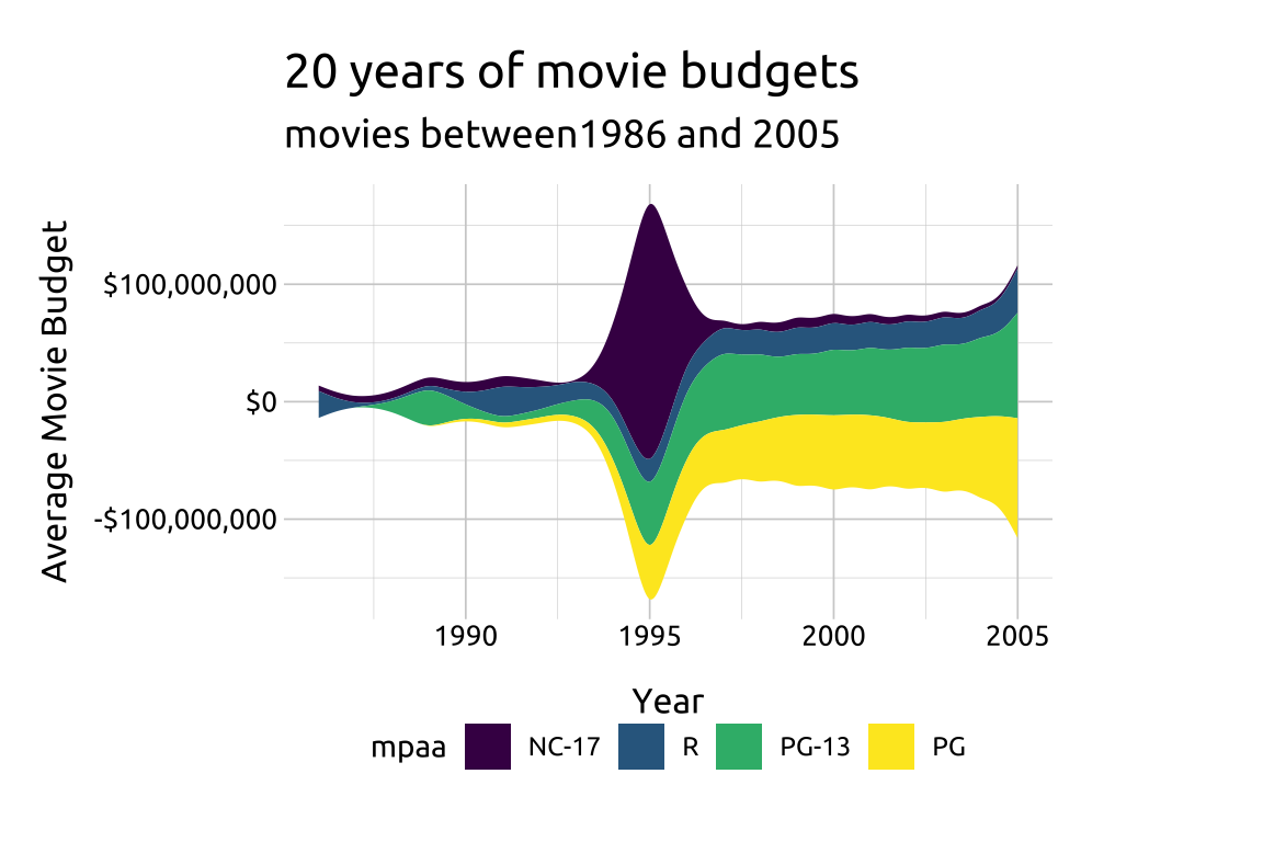
32.4.1 Type
Map
mpaatofill(wrapped inforcats::fct_rev())We can adjust the look of the graph by setting the
typeargument ingeom_stream()type: change type from"mirror"(the default) to"proportional"
Adjust colors:
scale_fill_manual(): Add colors as a named vector tovalues
Finally, add the
fillto the labels and move the legend withtheme(legend.position = "bottom")
show/hide
ggp2_stream_prp <- ggplot(data = movies_stream,
    mapping = aes(x = year,
                  y = avg_budget,
                  fill = forcats::fct_rev(mpaa))) +
    ggstream::geom_stream(type = "proportional") +
    scale_y_continuous(labels = scales::percent) +
  scale_fill_manual(
      values = c("PG-13" = "#0bd3d3",
                 "PG" = "#f890e7",
                 "R" = "#282b2d",
                 "NC-17" = "#772953"))
ggp2_stream_prp +
    labs_stream +
    labs(fill = "mpaa") +
    theme(legend.position = "bottom")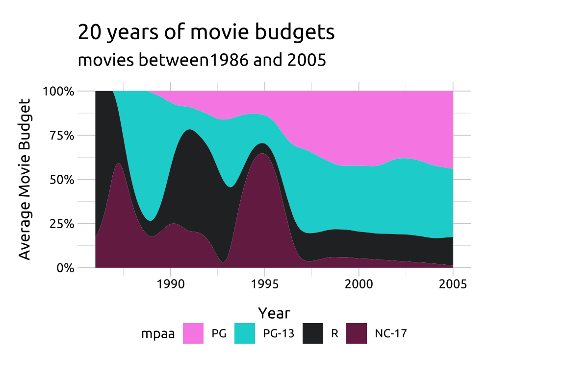
32.4.2 Sorting
To change how the categorical areas are sorted, adjust the sorting argument to either "none", "onset", or "inside_out"
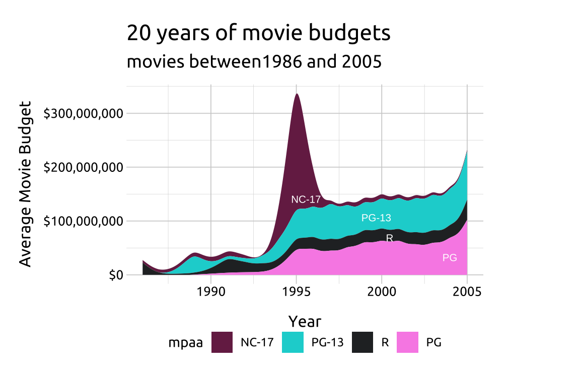
sorting: set thesortingmethod to"inside_out"in bothggstream::geom_stream()andggstream::geom_stream_label()type: change the type to"ridge"in bothggstream::geom_stream()andggstream::geom_stream_label()
We can also add text labels using ggstream::geom_stream_label():
Map
mpaa(wrapped inforcats::fct_rev()) tolabelgloballyInside
ggstream::geom_stream_label():set color to white (
"#ffffff") and thesizeto2.7Remove the legend with
show.legend = FALSE
Colors:
Use
scale_colour_manual()andscale_fill_manual()to manually set the values using a named vector- Change the
yaxis to US dollars usingscale_y_continuous()andscales::dollar
- Change the
Finally, add the
fillto the labels and move the legend withtheme(legend.position = "bottom")
show/hide
ggp2_stream_srt <- ggplot(data = movies_stream,
    mapping = aes(x = year,
                  y = avg_budget,
                  fill = fct_rev(mpaa),
                  label = fct_rev(mpaa))) +
    ggstream::geom_stream(
        type = "ridge",
        sorting = "inside_out") +
    ggstream::geom_stream_label(
        type = "ridge",
        sorting = "inside_out",
        color = "#ffffff",
        size = 2.7,
        show.legend = FALSE) +
    scale_colour_manual(
      values = c("PG-13" = "#0bd3d3",
                 "PG" = "#f890e7",
                 "R" = "#282b2d",
                 "NC-17" = "#772953")) +
    scale_fill_manual(
      values = c("PG-13" = "#0bd3d3",
                 "PG" = "#f890e7",
                 "R" = "#282b2d",
                 "NC-17" = "#772953")) +
    scale_y_continuous(labels = scales::dollar)

ggp2_stream_srt +
    labs_stream +
    labs(fill = "mpaa") +
    theme(legend.position = "bottom")