RELATIONSHIPS

Relationships: these graphs show how the change of values in variable x affect the values in variable y (and possibly z)?

Scatter plots

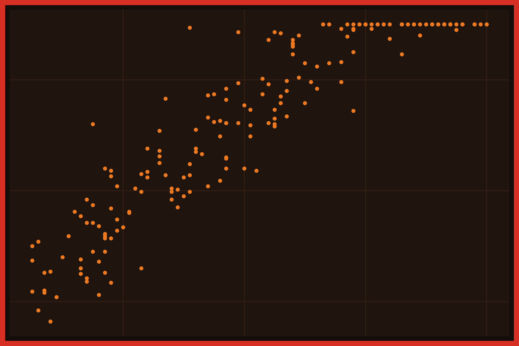
A scatter plot displays the relationship between two numeric variables, with one on the x axis and the other on the y axis. Each point is one observation, so the pattern of points shows whether the variables rise together, move in opposite directions, or aren’t related at all. Scatter plots also reveal clusters, outliers, and limits in the data. Transparency (alpha) helps when points overlap.

Grouped scatter plots

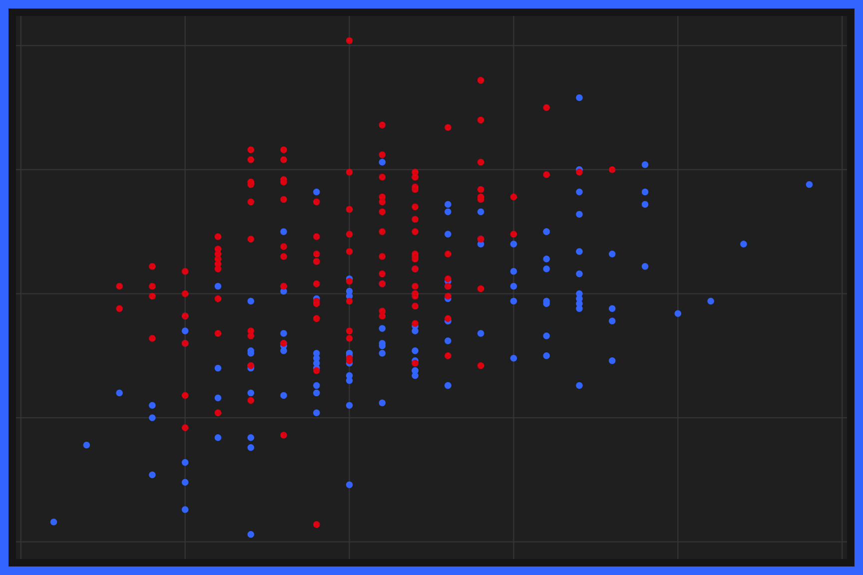
Grouped scatter plots display the relationship between two numeric variables across the levels of a categorical variable. Each group gets its own color (or shape), so we can compare the center, spread, and direction of each group’s cloud of points. Grouped scatter plots show whether the relationship is the same for every group. A legend explains the colors.

Bubble charts

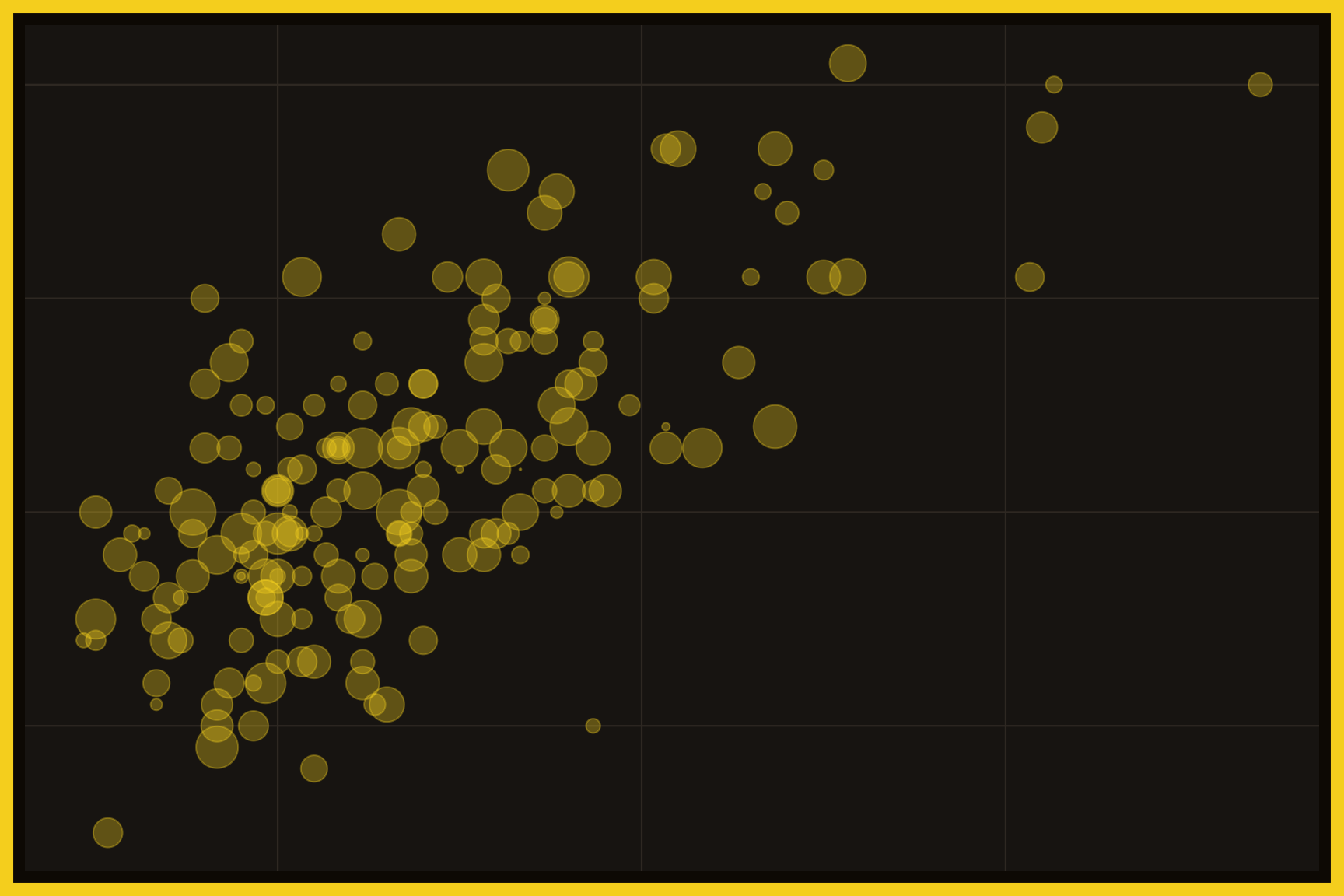
A bubble chart is a scatter plot with a third numeric variable mapped to the size of each point. The position of each bubble shows the first two variables, and its area shows the third. Bubble charts can display a lot of information at once, but overlapping bubbles may need transparency. A legend explains the bubble sizes.

Grouped bubble charts

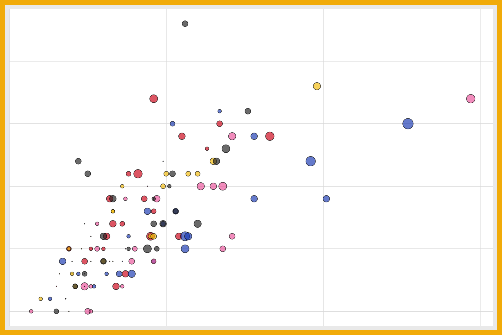
A grouped bubble chart adds a categorical variable to a bubble chart with color. Position shows two numeric variables, size shows a third, and color shows the group. Grouped bubble charts can compare several groups across three numeric variables in a single graph. Legends explain both the sizes and the colors.

Parallel sets

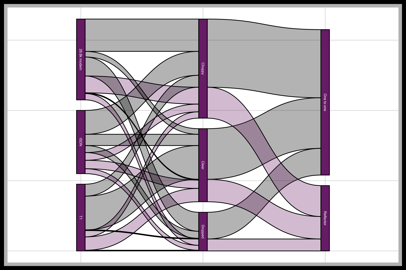
Parallel sets display the counts of several categorical variables as vertical axes connected by bands. Each band shows how many observations share a combination of categories, and its width is proportional to the count. Parallel sets show whether categorical variables are related, because related variables split into bands in different ways. Color usually follows one of the variables.

Density contours

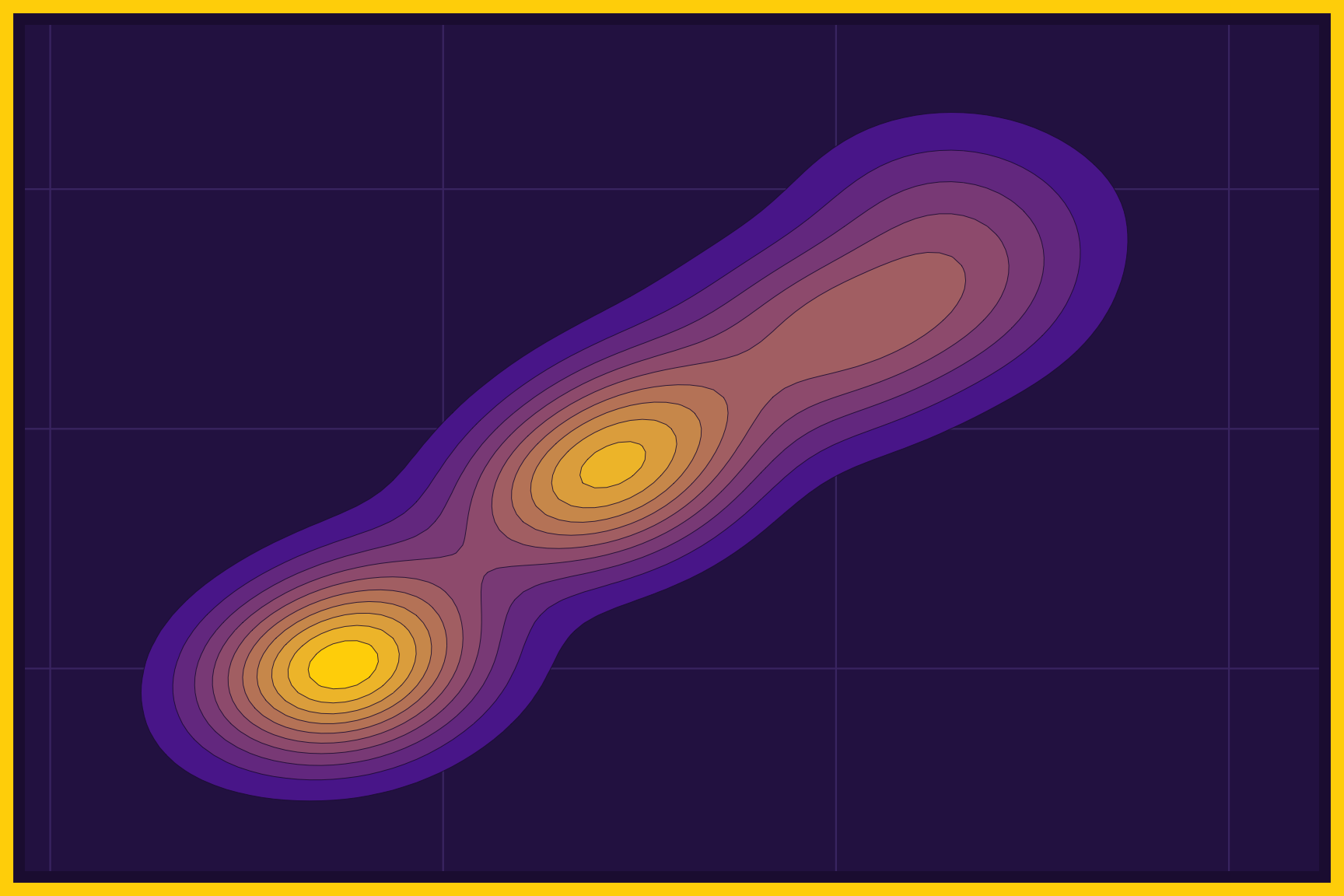
Density contours draw lines around the areas where the points in a scatter plot are most crowded, like the lines on a topographic map. The innermost contours surround the peaks, and filled contours use color to show the height of the density. Density contours are helpful when there are too many points to see in a scatter plot. A legend explains the contour levels.

2D histograms

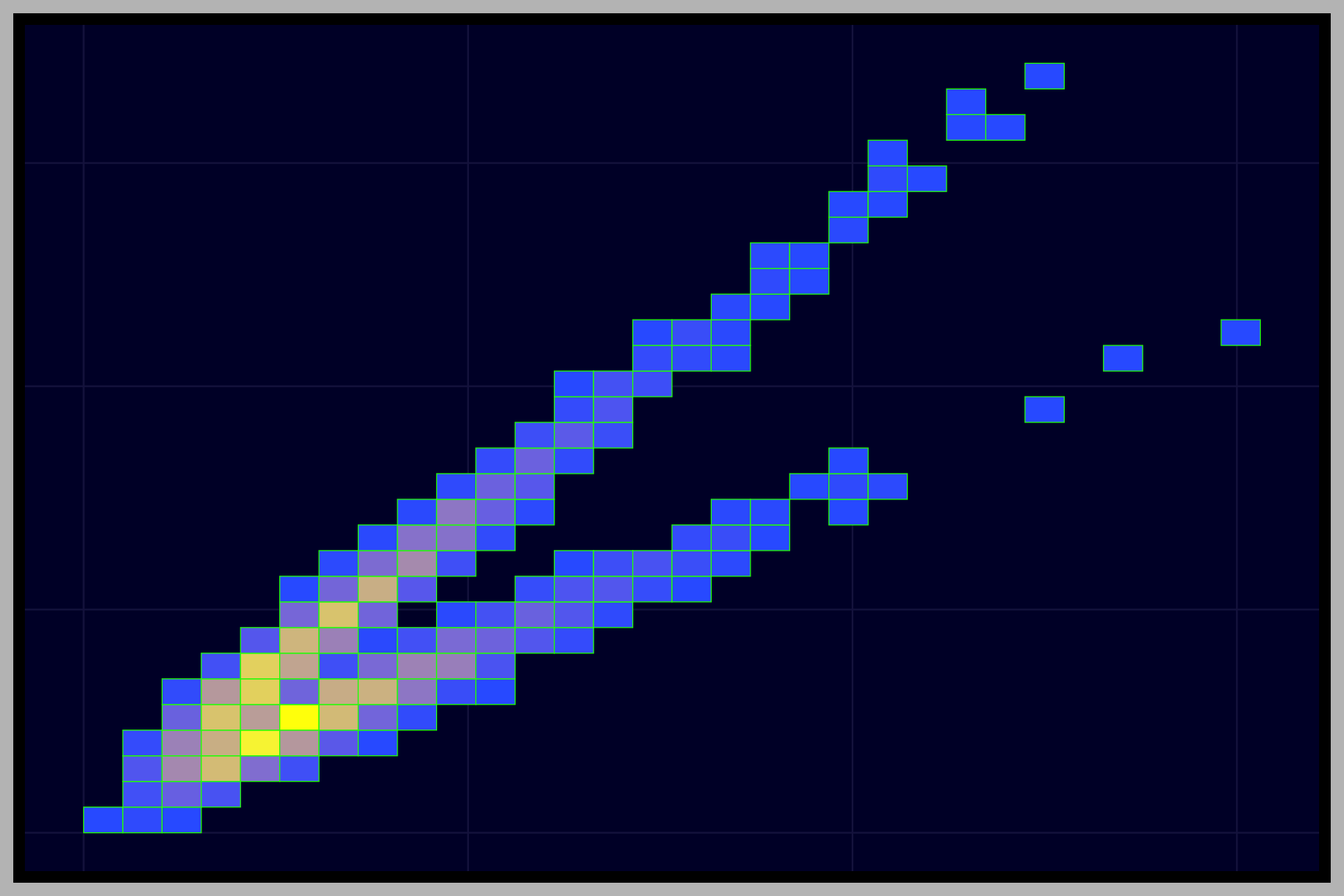
A 2D histogram divides the area of a scatter plot into a grid of squares and colors each square by how many points fall inside it. It extends the histogram to two numeric variables, and it works well for very large datasets. The size of the squares (set with bins) controls how much detail we see. A color scale explains the counts.

Hexagon bins

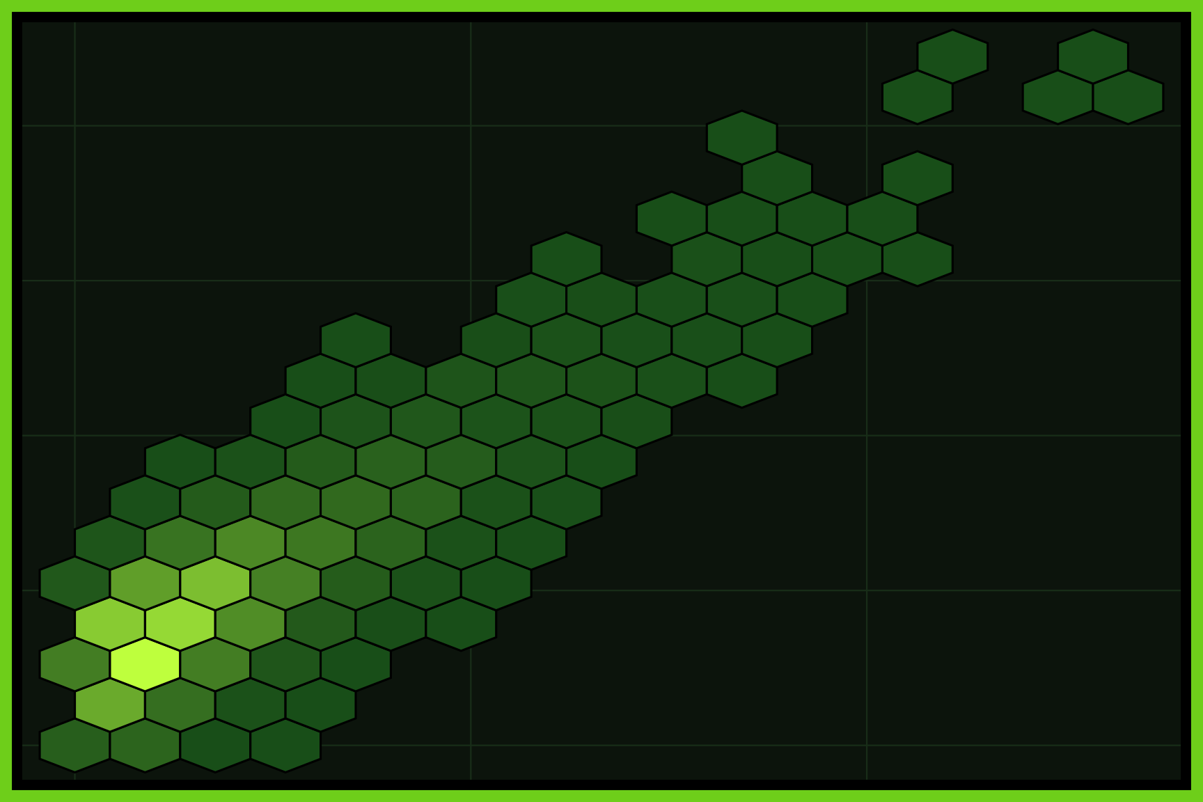
Hexagon bins work like a 2D histogram, but divide the graph area into hexagons instead of squares. Each hexagon is colored by the number of points inside it, and hexagons fit together without the corners of a square grid. Hexagon bins are another good choice for large datasets with lots of overplotting. A color scale explains the counts.