10  Overlapping bar graphs

This graph requires:

✅ a numeric (continuous) variable

✅ a categorical variable

10.1 Desription

Overlapping bar graphs display multiple variables on the same graph. Bars overlap instead of being placed side by side. Bars are often made partially transparent to aid visibility. A legend is essential to distinguish between data.

In ggplot2, we can build overlapping bar graphs using the fill argument in geom_bar() or geom_col()

10.2 Set up

PACKAGES:

Install packages.

install.packages("palmerpenguins")
library(palmerpenguins)
library(ggplot2)

DATA:

Artwork by Allison Horst

Remove missing species from penguins and filter the data to only penguins on "Dream" island.

penguins_ovrlp <- filter(penguins,
                      !is.na(species) & 
                            island == "Dream")
glimpse(penguins_ovrlp)
#> Rows: 124
#> Columns: 8
#> $ species           <fct> Adelie, Adelie, Adelie…
#> $ island            <fct> Dream, Dream, Dream, D…
#> $ bill_length_mm    <dbl> 39.5, 37.2, 39.5, 40.9…
#> $ bill_depth_mm     <dbl> 16.7, 18.1, 17.8, 18.9…
#> $ flipper_length_mm <int> 178, 178, 188, 184, 19…
#> $ body_mass_g       <int> 3250, 3900, 3300, 3900…
#> $ sex               <fct> female, male, female, …
#> $ year              <int> 2007, 2007, 2007, 2007…

10.3 Grammar

CODE:

• Create labels with labs()

• Initialize the graph with ggplot() and provide data

• Map flipper_length_mm to the x and species to fill

• Add the geom_bar() layer

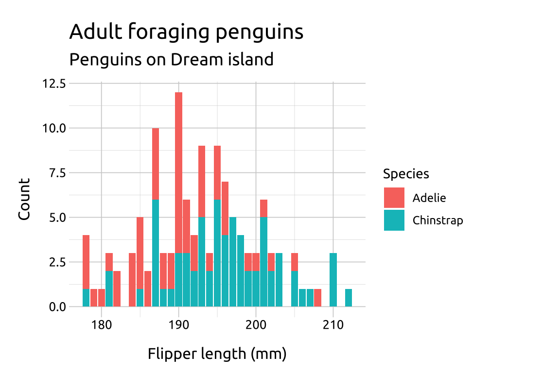
labs_bar_ovrlp <- labs(
  title = "Adult foraging penguins on Dream island",
  x = "Flipper length (mm)",
  y = "Count",
  fill = "Species")
ggp2_bar_ovrlp <- ggplot(data = penguins_ovrlp,
          aes(x = flipper_length_mm, fill = species)) +
                geom_bar() 
ggp2_bar_ovrlp + 
  labs_bar_ovrlp

GRAPH:

10.4 More info

• Overlapping bar graphs can also be built with geom_col().

• geom_bar() has additional options for arranging overlapping bars. We can set the position argument to "dodge" or "dodge2", depending on how we’d like the data displayed.

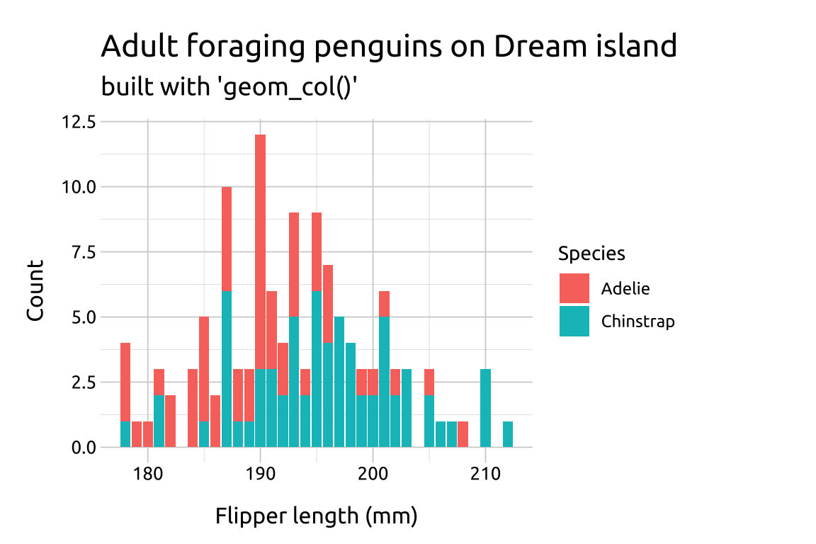
10.4.1 geom_col()

To build an overlapping bar graph with geom_col(), we need to create a column with the counts for flipper_length_mm and species in the dataset.

• Create the penguins_col data:

penguins_col <- penguins_ovrlp |>
    count(species, flipper_length_mm, name = "Count")

• Map the counts to the y axis, flipper_length_mm to the x axis, and species to fill

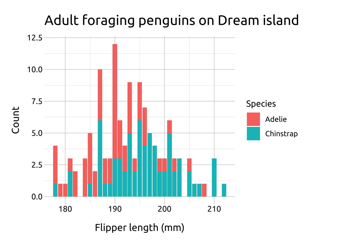
labs_col_ovrlp <- labs(
  title = "Adult foraging penguins on Dream island",
  subtitle = "built with 'geom_col()'",
  x = "Flipper length (mm)",
  y = "Count",
  fill = "Species")
ggp2_col_ovrlp <- ggplot(data = penguins_col, 
    mapping = aes(y = Count, 
        x = flipper_length_mm, 
        fill = species)) + 
    geom_col()
ggp2_col_ovrlp + 
    labs_col_ovrlp

Compare the two graphs below:

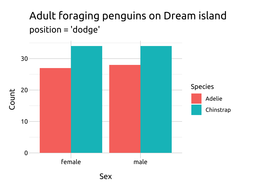
10.4.2 dodge

• position = "dodge" preserves the vertical position of a geom while adjusting the horizontal position

• "dodge" requires the grouping variable to be be specified in the global or ⁠geom_⁠ layer

Create the penguins_dodge data.

penguins_dodge <- filter(penguins,
                      !is.na(species) & 
                        !is.na(sex) &
                            island == "Dream")
glimpse(penguins_dodge)
#> Rows: 123
#> Columns: 8
#> $ species           <fct> Adelie, Adelie, Adelie…
#> $ island            <fct> Dream, Dream, Dream, D…
#> $ bill_length_mm    <dbl> 39.5, 37.2, 39.5, 40.9…
#> $ bill_depth_mm     <dbl> 16.7, 18.1, 17.8, 18.9…
#> $ flipper_length_mm <int> 178, 178, 188, 184, 19…
#> $ body_mass_g       <int> 3250, 3900, 3300, 3900…
#> $ sex               <fct> female, male, female, …
#> $ year              <int> 2007, 2007, 2007, 2007…

• Create labels with labs()

• Initialize the graph with ggplot() and provide data

• Map species to the x and island to group and fill

• Inside the geom_bar() function, set position to "dodge"

labs_bar_dodge <- labs(
  title = "Adult foraging penguins on Dream island",
  subtitle = "position = 'dodge'",
  x = "Sex",
  y = "Count",
  fill = "Species")
ggp2_bar_dodge <- ggplot(data = penguins_dodge,
                    aes(x = sex, 
                        group = species, 
                        fill = species)) +
                    geom_bar(
                        position = "dodge")
ggp2_bar_dodge +
  labs_bar_dodge

10.4.3 dodge2

• Create labels with labs()

• Initialize the graph with ggplot() and provide data

• Map species to x and island to fill

• Inside geom_bar(), set position to "dodge2"

• "dodge2" works without a grouping variable in a layer

• "dodge2" works with bars and rectangles

• "dodge2" is useful for arranging graphs with variable widths.

labs_bar_dodge2 <- labs(
  title = "Adult foraging penguins on Dream island",
  subtitle = "position = 'dodge2'",
  x = "Sex",
  y = "Count",
  fill = "Species")
ggp2_bar_dodge2 <- ggplot(data = penguins_dodge,
                    aes(x = sex, 
                        fill = species)) +
                    geom_bar(
                        position = "dodge2")
ggp2_bar_dodge2 +
  labs_bar_dodge2

Compare the two graphs below: