16  Mosaic plots

This graph is largely complete and just needs final proof reading.

This graph requires:

✅ at least two categorical variables

16.1 Description

A mosaic plot is similar to a stacked bar graph, but instead of only relying on height and color to display the relative amount for each value, mosaic plots also use width.

Mosaic plot legends should be positioned on top or bottom and justified horizontally to preserve shape and improve readability.

We can build mosaic plots using the ggmosaic package.

16.2 Set up

PACKAGES:

Install packages.

install.packages("fivethirtyeight")
library(fivethirtyeight) 
# pak::pak("haleyjeppson/ggmosaic")
library(ggmosaic)
library(ggplot2)

DATA:

For this graph, we’ll be using the fivethirtyeight::flying dataset, after removing the missing values from baby, recline_rude, and unruly_child.

fly_mosaic <- fivethirtyeight::flying |> 
                dplyr::select(baby, unruly_child, recline_rude) |> 
                tidyr::drop_na()
glimpse(fly_mosaic)
#> Rows: 849
#> Columns: 3
#> $ baby         <ord> No, Somewhat, Somewhat, Som…
#> $ unruly_child <ord> No, Very, Very, Very, Very,…
#> $ recline_rude <ord> Somewhat, No, No, No, No, S…

16.3 Grammar

CODE:

• Create labels with labs()

• Initialize the graph with ggplot() and provide data

• Map the product() of unruly_child and baby to the x axis

• Map baby to fill

• Add theme_mosaic()

• Move the legend to the bottom with theme(legend.position = "bottom")

labs_mosaic <- labs(
      title = "In general...", 
      subtitle = "...is it rude to...",
      x = "... bring a baby on a plane?",
      y = "...knowingly bring unruly children on a plane?",
      fill = "Response") 
ggp2_mosaic <- ggplot(data = fly_mosaic) +
   ggmosaic::geom_mosaic(mapping = 
          aes(x = product(unruly_child, baby), 
              fill = baby)) + 
    ggmosaic::theme_mosaic(base_size = 10) + 
    theme(legend.position = "bottom")
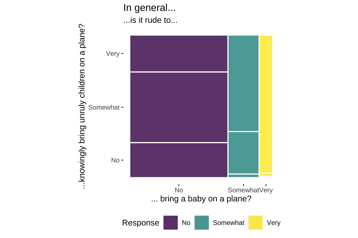
ggp2_mosaic + 
    labs_mosaic

GRAPH:

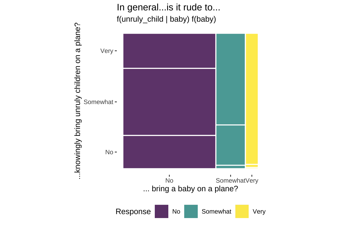
16.3.1 Details

We’ve re-written the labels for the mosaic plot (ggp2_mosaic) to illustrate what’s happening in the aes() of geom_mosaic().

It’s a good idea to adjust the fig-height and fig-width of your graph

The table below displays the counts for each combined response. As we can see, the counts are represented by height and width in the graph.

unruly_child	No	Somewhat	Very
Very	152	125	74
Somewhat	296	54	1
No	144	3

16.4 More info

I recommend reading the ggmosaic vignette, particularly the sections on ordering and conditioning.

16.4.1 Two variables

unruly_child	No	Somewhat	Very
Very	193	119	39
Somewhat	204	123	24
No	102	38	7

Below is another example of a two-variable mosaic plot, mapping the product() variables as unruly_child and recline_rude, and the fill variable as recline_rude.

Once again we can see the counts for each category in the cross-tabulation:

# build 2-variable mosiac plot
labs_mosaic_2var <- labs(
  title = "In general...is it rude to...", 
  subtitle = "2-Variable plot",
  x = "... recline your seat on a plane?",
  y = "...knowingly bring unruly children on a plane?",
  fill = "recline_rude responses")

ggp2_mosaic_2var <- ggplot(data = fly_mosaic) +
  geom_mosaic(aes(
    x = product(unruly_child, recline_rude),
    fill = recline_rude)) +
  ggmosaic::theme_mosaic(base_size = 10) + 
  theme(legend.position = "bottom")
  
ggp2_mosaic_2var + 
    labs_mosaic_2var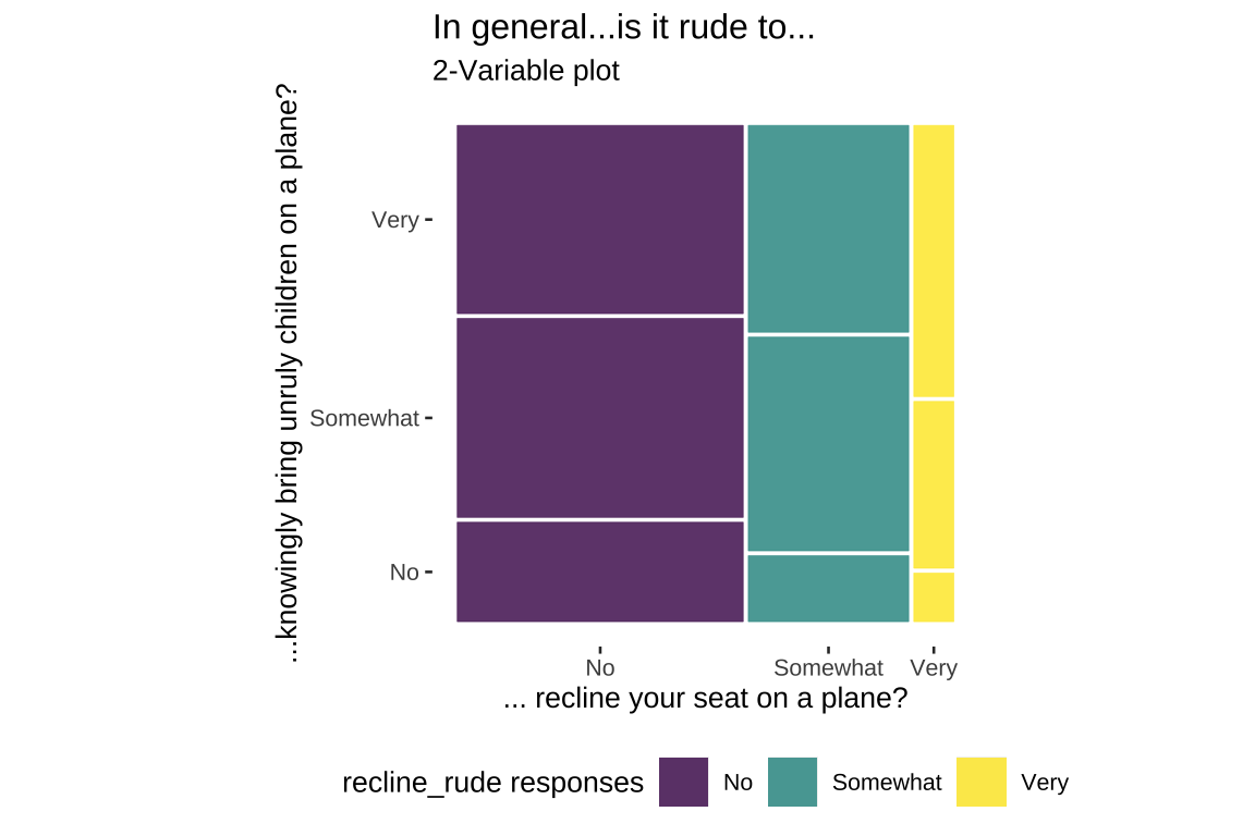

For conditional variables, we map the product() variable as unruly_child and the fill variable as baby, but include a conds variable (as product(recline_rude)).

# build conditional mosiac plot
labs_mosaic_cond <- labs(
  title = "In general...is it rude to...", 
  subtitle = "Conditional plot",
  x = "...recline your seat on a plane?",
  y = "...knowingly bring unruly children on a plane?",
  fill = "unruly_child responses")
ggp2_mosaic_cond <- ggplot(data = fly_mosaic) +
  geom_mosaic(aes(
    x = product(unruly_child), # product variable
    fill = unruly_child,
    conds = product(recline_rude))) + # conditional variable
  ggmosaic::theme_mosaic(base_size = 10) + 
  theme(legend.position = "bottom")

ggp2_mosaic_cond + 
    labs_mosaic_cond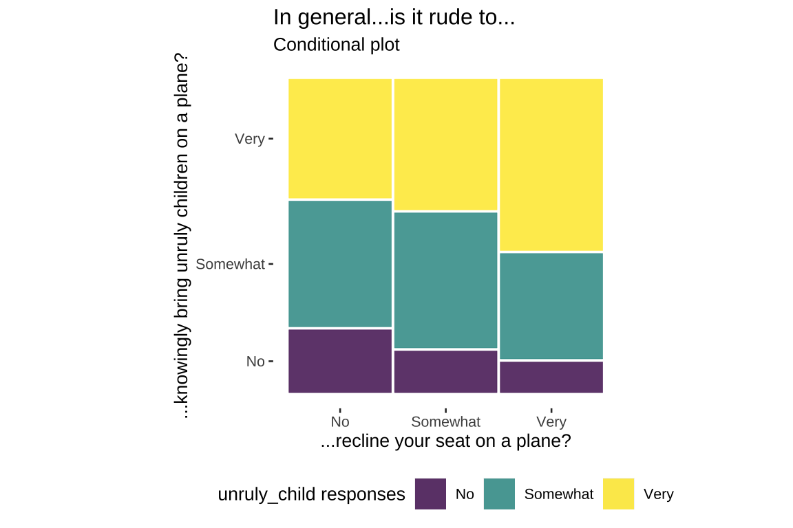

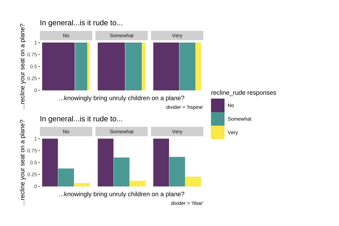
16.4.2 Facets

Another option for including a conditioning variable is including facets. In the example below we use recline_rude in both x and fill (remember to wrap recline_rude in product()).

The divider argument let’s us control the spine partitions (vertically and horizontally). Below are the two vertical orientation options for the divider argument.

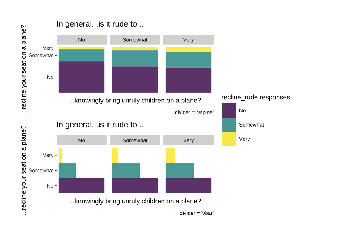
The two horizontal orientation options make the axis text harder to read, so these need to be manipulated manually.