22  Beeswarm plots

This graph is largely complete and just needs final proof reading.

This graph requires:

✅ a categorical variable

✅ a numeric (continuous) variable

22.1 Description

The beeswarm plot uses points to display the distribution of a continuous variable across the levels of a categorical variable.

The points are grouped by level, and the shape (or swarm) of the distribution is mirrored above and below the quantitative axis (similar to a violin plot).

We can create beeswarm plot using geom_jitter() or the ggbeeswarm package.

22.2 Set up

PACKAGES:

Install packages.

# pak::pak("eclarke/ggbeeswarm")
library(ggbeeswarm)
install.packages("palmerpenguins")
library(palmerpenguins) 
library(ggplot2)

DATA:

Artwork by allison horst

Create peng_beeswarm by grouping penguins by species, then calculating the bill_ratio (bill_length_mm / bill_depth_mm), and then removing any missing values from bill_ratio

peng_beeswarm <- palmerpenguins::penguins |> 
    dplyr::group_by(species) |> 
    dplyr::mutate(bill_ratio = bill_length_mm / bill_depth_mm) |>  
    dplyr::filter(!is.na(bill_ratio)) |> 
    dplyr::ungroup()
glimpse(peng_beeswarm)
#> Rows: 342
#> Columns: 9
#> $ species           <fct> Adelie, Adelie, Adelie…
#> $ island            <fct> Torgersen, Torgersen, …
#> $ bill_length_mm    <dbl> 39.1, 39.5, 40.3, 36.7…
#> $ bill_depth_mm     <dbl> 18.7, 17.4, 18.0, 19.3…
#> $ flipper_length_mm <int> 181, 186, 195, 193, 19…
#> $ body_mass_g       <int> 3750, 3800, 3250, 3450…
#> $ sex               <fct> male, female, female, …
#> $ year              <int> 2007, 2007, 2007, 2007…
#> $ bill_ratio        <dbl> 2.090909, 2.270115, 2.…

22.3 Grammar

CODE:

• Create labels with labs()

• Initialize the graph with ggplot() and provide data

• Map species to the x axis and color

• Map bill_ratio to the y axis

• Add the ggbeeswarm::geom_beeswarm() layer (with alpha)

• Remove the legend with show.legend = FALSE

labs_beeswarm <- labs(
    title = "Adult Foraging Penguins",
    subtitle = "Bill Length (mm) / Bill Depth (mm) = Bill Ratio",
    x = "Species",
    y = "Bill Ratio")
ggp2_beeswarm <- ggplot(data = peng_beeswarm,
    aes(x = species,
        y = bill_ratio,
        color = species)) +
    ggbeeswarm::geom_beeswarm(alpha = 2 / 3,
        show.legend = FALSE)
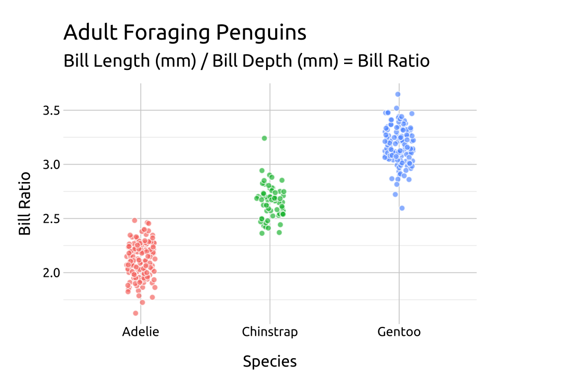
ggp2_beeswarm +
    labs_beeswarm

GRAPH:

Adjust the size/shape of the swarm using method = or the geom_quasirandom() function

22.4 More info

Below is some additional arguments and methods for beeswarm plots.

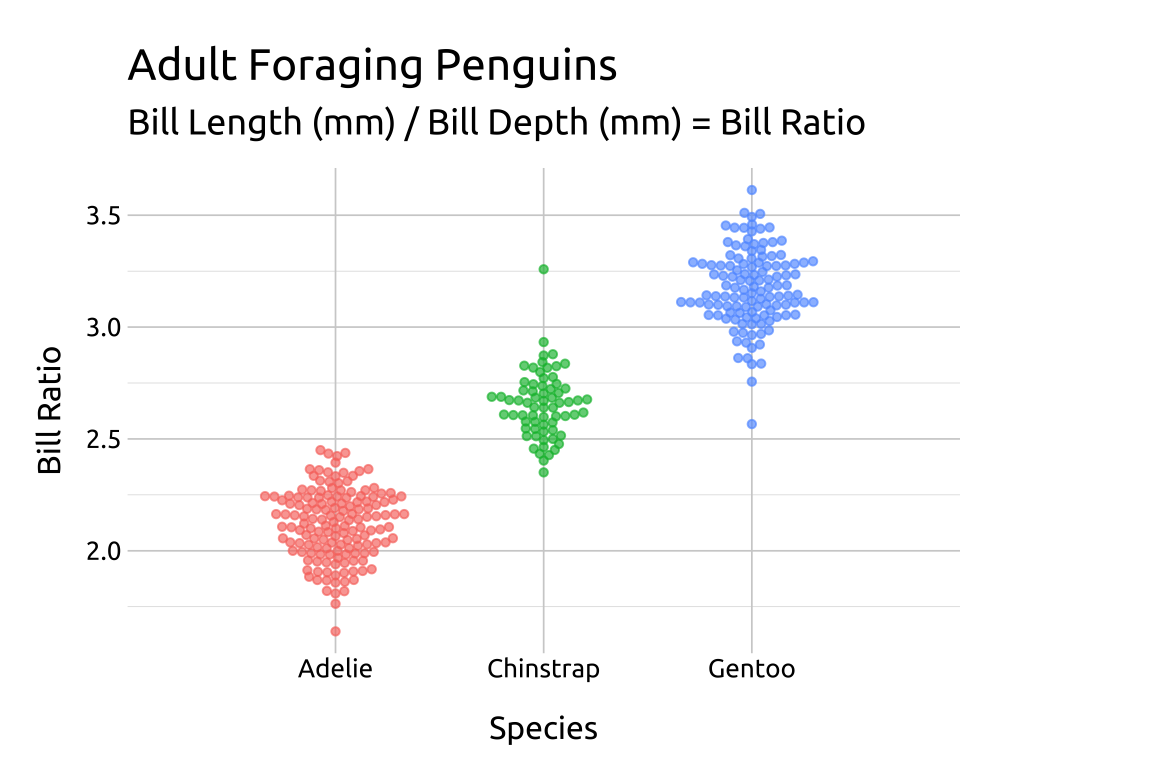
22.4.1 method

Use method to adjust the shape of the beeswarm (swarm, compactswarm, hex, square, center, or centre)

Set the point shape to 21 to control the fill and color

ggp2_compact_swarm <- ggplot(data = peng_beeswarm,
    mapping = aes(x = species,
                  y = bill_ratio,
                color = species)) +
    ggbeeswarm::geom_beeswarm(
      aes(fill = species),
        method = 'compactswarm', 
        dodge.width = 0.5,
        shape = 21,
        color = "#ffffff",
        alpha = 2/3, size = 1.7,
        show.legend = FALSE) 
ggp2_compact_swarm + 
    # add labels
    labs_beeswarm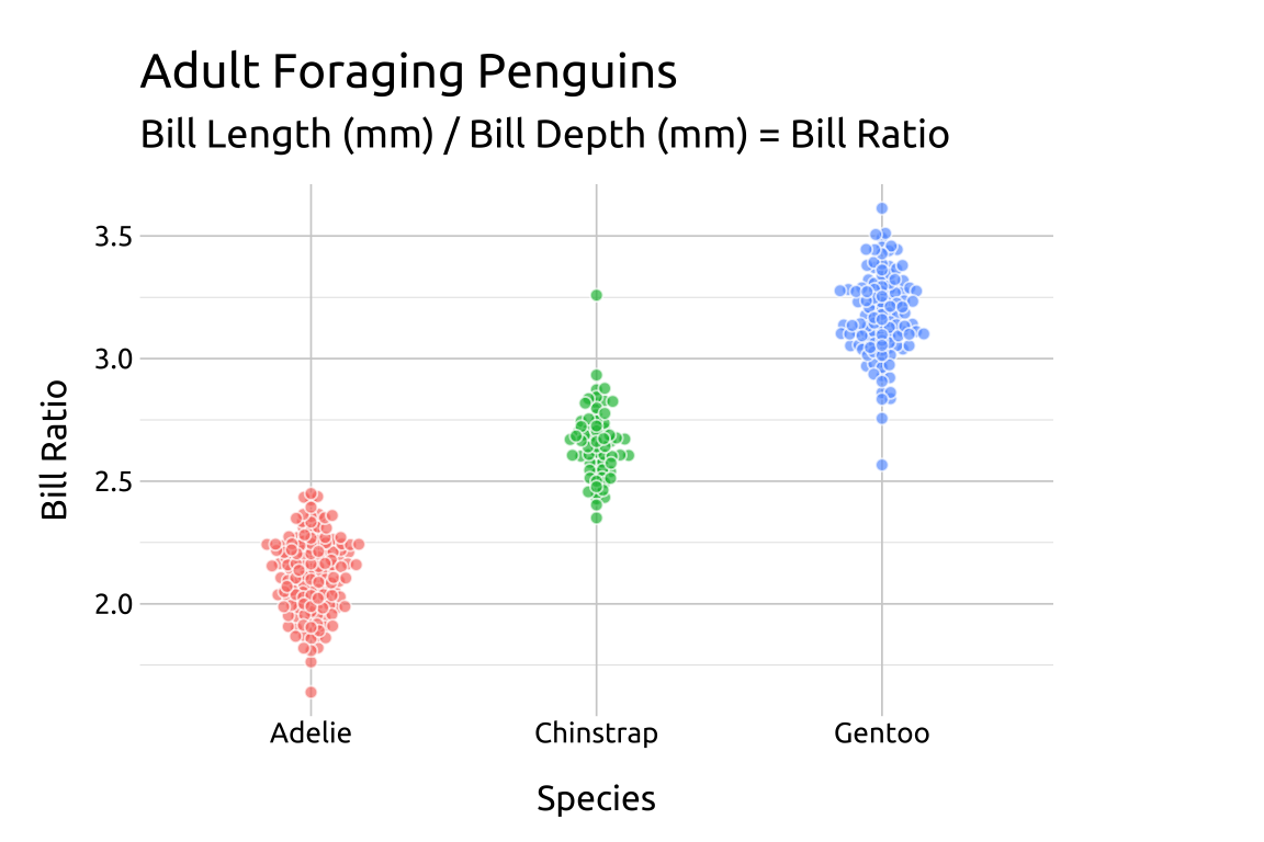

22.4.2 side

For a beeswarm that falls across the vertical axis, use the side argument.

ggp2_rside_swarm <- ggplot(data = peng_beeswarm,
    mapping = aes(x = species,
                  y = bill_ratio,
                color = species)) +
    ggbeeswarm::geom_beeswarm(
      aes(fill = species),
        side = 1, # right/upwards
        shape = 21,
        color = "#ffffff",
        alpha = 2/3, 
        size = 1.7,
        show.legend = FALSE) 
ggp2_rside_swarm + 
    # add labels
    labs_beeswarm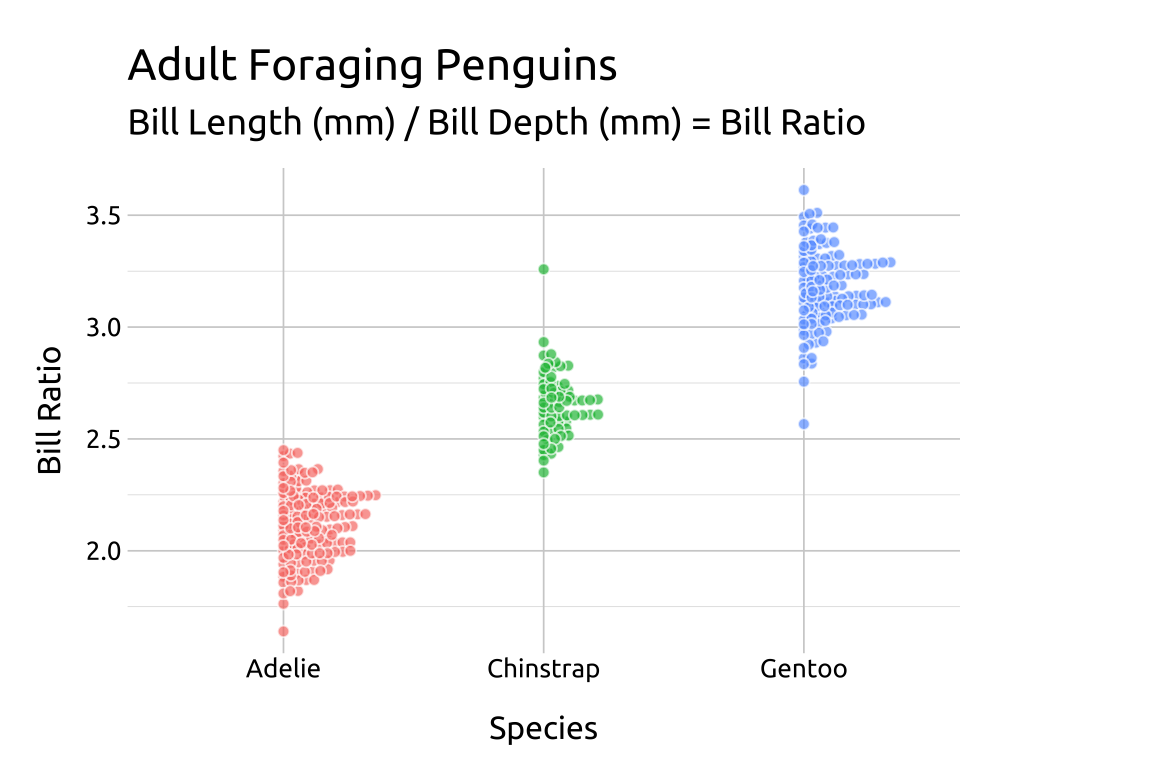

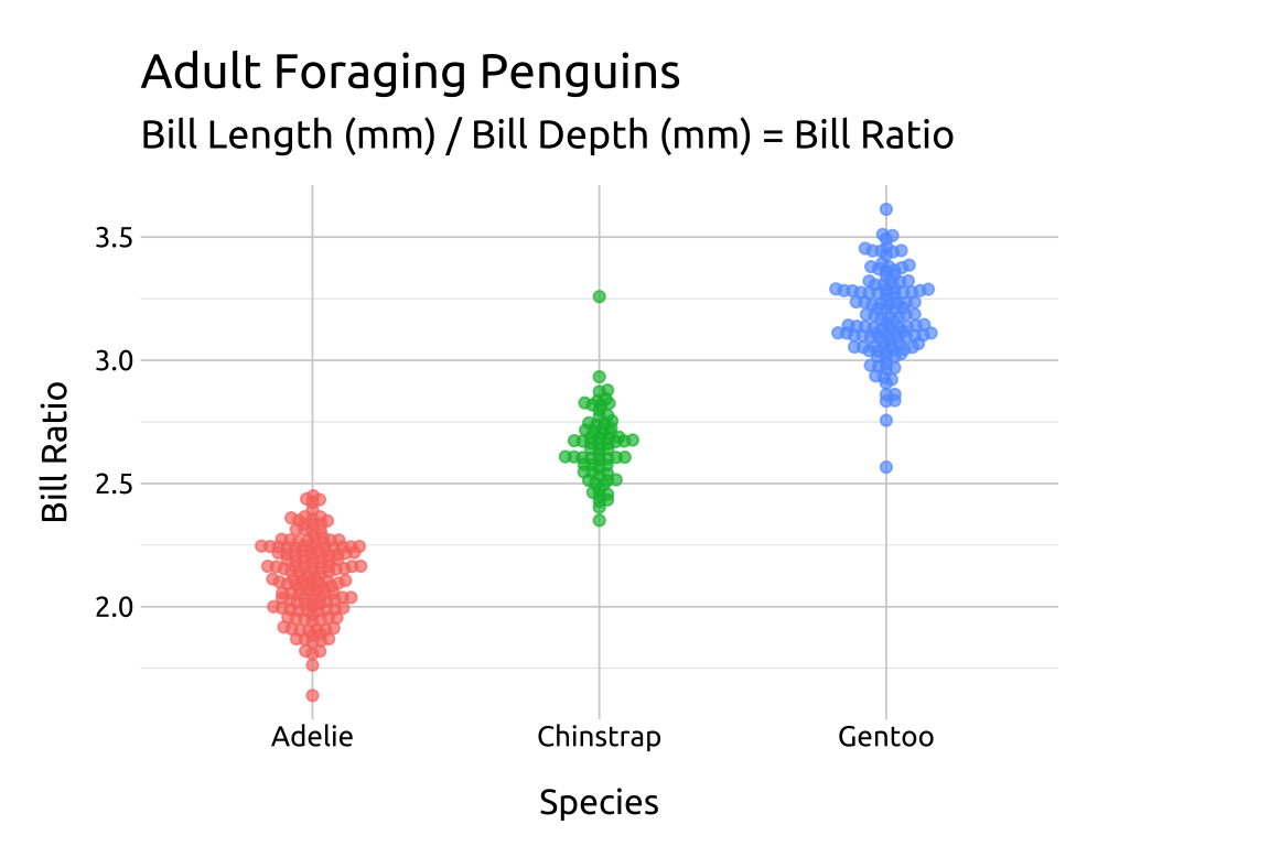
22.4.3 cex

The cex argument controls the “scaling for adjusting point spacing”

ggp2_beeswarm_cex <- ggplot(data = peng_beeswarm,
    mapping = aes(x = species,
                  y = bill_ratio,
                color = species)) +
    ggbeeswarm::geom_beeswarm(
      aes(fill = species),
        cex = 1.6,
        shape = 21,
        color = "#ffffff",
        alpha = 2/3, 
        size = 1.7,
        show.legend = FALSE) 
ggp2_beeswarm_cex + 
    # add labels
    labs_beeswarm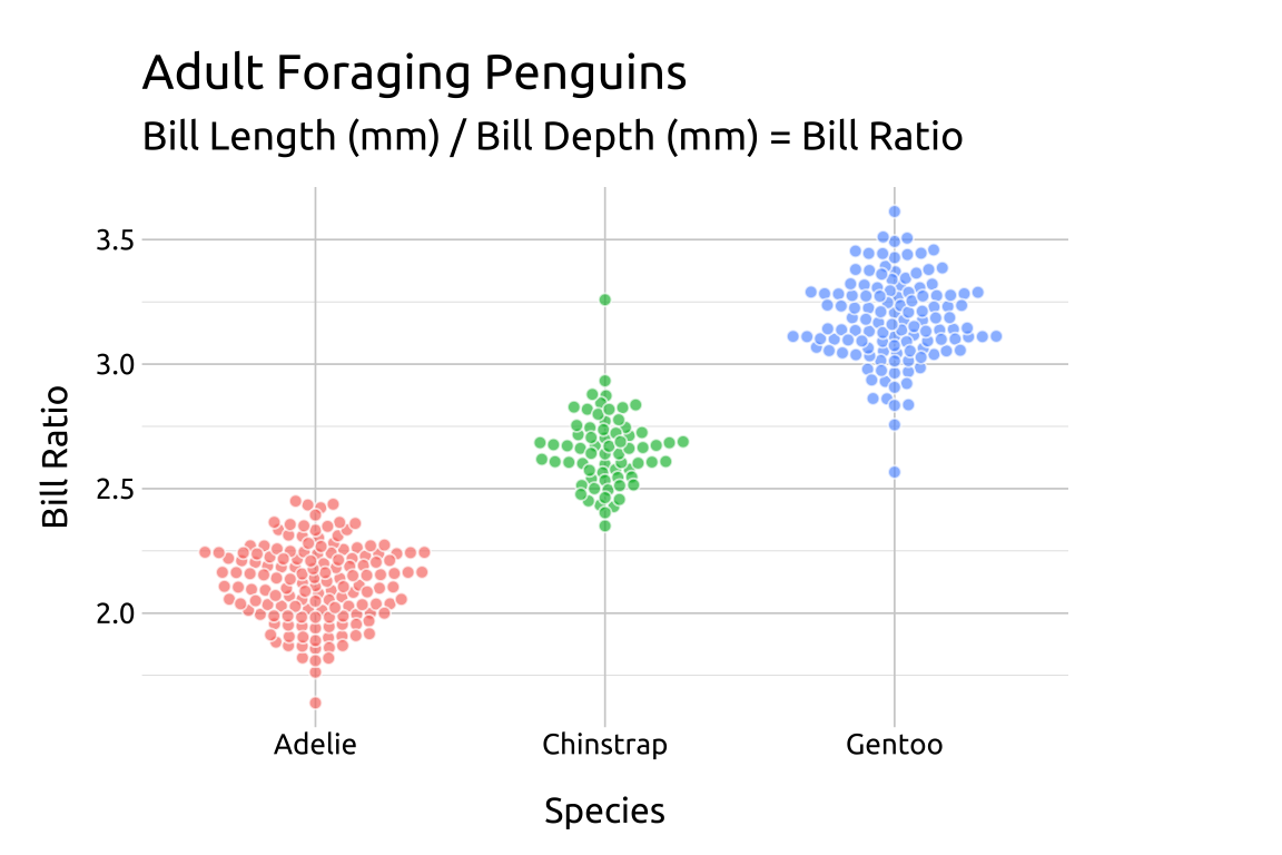

22.4.4 geom_jitter()

We can also create a beeswarm using the geom_jitter() and setting the height and width.

ggp2_jitter_swarm <- ggplot(data = peng_beeswarm,
    mapping = aes(x = species,
        y = bill_ratio,
        color = species)) +
    geom_jitter(
        aes(fill = species),
        height = 0.05,
        width = 0.11,
        shape = 21,
        color = "#ffffff",
        alpha = 2 / 3,
        size = 1.7,
        show.legend = FALSE)
ggp2_jitter_swarm + 
    # add labels
    labs_beeswarm